Using Data Forms

A data form is used to allow easy manipulation of information in an Excel data list. While a list is small—for instance, when it fits on one screen—it is easier to enter or change information directly. When you start getting a larger number of records, then you may find using a data form to be easier.

A data form is a dialog box that displays one complete record from your list at a time. Excel considers a record to be a single row in your data list, so a data form basically extracts the information from a row, uses the field labels from the first row of the list, and displays the information so you can understand it easier.

In earlier versions of Excel (before Excel 2007), data forms held a more conspicuous position, as they could easily be accessed from the available menus. The data form command is no longer available on Excel's ribbons, but that doesn't change the fact that they can be valuable for working with some types of data. Fortunately, Excel allows you to add the primary data form command to the Quick Access Toolbar. Follow these steps:

1. Display the Excel Options dialog box. (In Excel 2007 click the Office button and then click Excel Options. In Excel 2010 or later versions, display the File tab of the ribbon and then click Options.)
2. At the left side of the dialog box, click Customize (Excel 2007) or Quick Access Toolbar (Excel 2010 or later versions). (See Figure 1.)



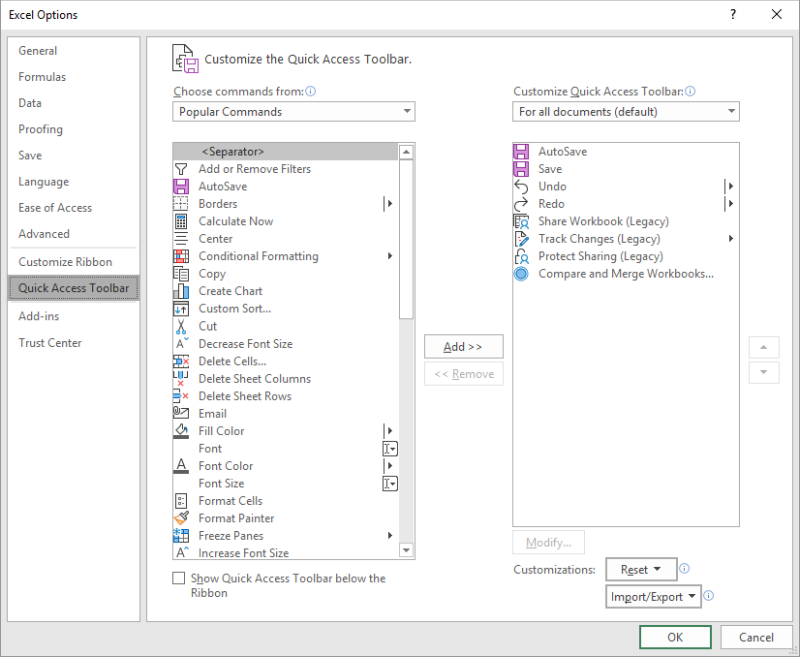
Figure 1. The Quick Access Toolbar option of the Excel Options dialog box.

3. Using the Choose Commands From drop-down list, choose Commands Not in the Ribbon.
4. Scroll through the list of commands and select the Form command.
5. Click the Add button. The Form command now appears at the right side of the dialog box.
6. Click OK. The Form command now appears on the Quick Access Toolbar.

You can now use a data form by selecting any cell within your data list and clicking the Form icon on the Quick Access Toolbar. A data form appears. (See Figure 2.)

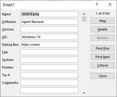
Figure 2. A sample data form.

There are several important items to note when working with data forms. The title that appears at the top of the data form is taken directly from the name of the worksheet on which the data resides. If you want to change the title, simply change the name of the worksheet tab.

The field labels are listed down the left side, and you can input information to the right of these labels. If a field contains a formula, you cannot enter information in that field; it is calculated automatically.

You can move between entry fields by pressing the Tab key. When you press Enter, any changes you make are saved in the record. The buttons at the right side of the data form are used to navigate through the list. If you click your mouse on the Close button, the data form is removed and you are returned to your worksheet.

Notice that there are several searching buttons located along the right side of the data form. The Find Prev and Find Next buttons are used to step through your list. If you click on the Criteria button, you can enter information that will be used by the other search buttons (Find Prev and Find Next) when displaying records.

Data forms have some drawbacks which some people find objectionable. (The pros and cons of data forms is beyond the scope of this tip.) That doesn't change the fact that for some people with some types of data, using a data form can be very handy and adding the Form tool to the Quick Access Toolbar can give back a functionality that, at first blush, seems missing in the latest versions of Excel.

ExcelTips is your source for cost-effective Microsoft Excel training. This tip (6207) applies to Microsoft Excel 2007, 2010, 2013, 2016, 2019, and Excel in Microsoft 365. You can find a version of this tip for the older menu interface of Excel here: Using Data Forms.