Formatting Subtotal Rows

When you add subtotals to a worksheet, Excel automatically formats the subtotals using a bold font. You, however, may want to have some different type of formatting for the subtotals, such as shading them in yellow or a different color.

If you use subtotals sparingly, and only want to apply a different format for one or two worksheets, you can follow these general steps:

1. Apply your subtotals, as desired.
2. Select the entire data table, including the subtotals.
3. Using the Outline area at the left of the screen, collapse the detail in your worksheet so that only the subtotals are showing.
4. Press F5 to display the Go To dialog box. (See Figure 1.)



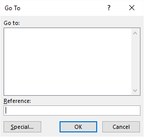
Figure 1. The Go To dialog box.

5. Click Special to display the Go To Special dialog box. (See Figure 2.)



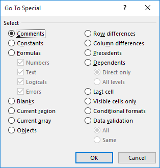
Figure 2. The Go To Special dialog box.

6. Select the Visible Cells Only option button.
7. Click OK. Now, only the visible subtotal rows are selected.
8. Apply your formatting, as desired.

If you will be repeatedly adding and removing subtotals to the same data table, you may be interested in using conditional formatting to apply the desired subtotal formatting. Follow these steps:

1. Before applying your subtotals, select your entire data table.
2. Make sure the Home tab of the ribbon is displayed.
3. Click the Conditional Formatting tool. Excel displays a series of choices.
4. Click Manage Rules. Excel displays the Conditional Formatting Rules Manager dialog box.
5. Click New Rule. Excel displays the New Formatting Rule dialog box. (See Figure 3.)



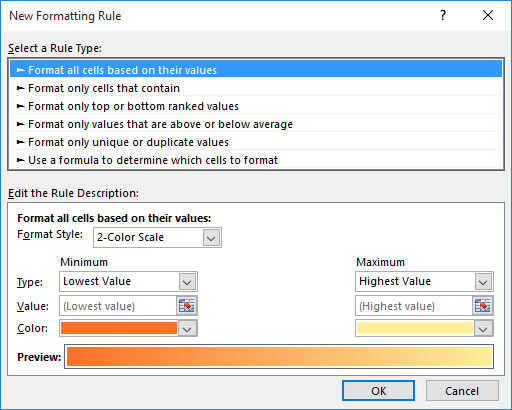
Figure 3. The New Formatting Rule dialog box.

6. In the Select a Rule Type area at the top of the dialog box, choose Use a Formula to Determine Which Cells to Format. Excel changes the appearance of the New Formatting Rule dialog box.
7. In the formula space, enter the following formula: =ISNUMBER(FIND("Grand Total",$A1))
8. Click Format to display the Format Cells dialog box.
9. Using the controls in the dialog box, set the formatting as you want it applied to the Grand Total row.
10. Click OK to dismiss the Format Cells dialog box.
11. Click OK to dismiss the New Formatting Rule dialog box. The rule you just created now appears in the Conditional Formatting Rules Manager dialog box.
12. Click New Rule. Excel again displays the New Formatting Rule dialog box.
13. In the Select a Rule Type area at the top of the dialog box, choose Use a Formula to Determine Which Cells to Format.
14. In the formula box, enter the following formula: =ISNUMBER(FIND("Total",$A1))
15. Click Format to display the Format Cells dialog box. (See Figure 4.)



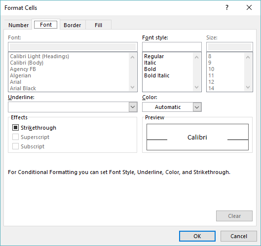
Figure 4. The Format Cells dialog box.

16. Using the controls in the dialog box, set the formatting as you want it applied to the Total row.
17. Click OK to dismiss the Format Cells dialog box.
18. Click OK to dismiss the New Formatting Rule dialog box.
19. Click the up and down arrows to move the rules you created to the order in which they should be evaluated.
20. Click OK to dismiss the Conditional Formatting Rules Manager dialog box.

When following the above steps, make sure that you replace A1 (steps 7 and 14) with the column in which your subtotals are added. Thus, if your subtotals are in column G, you would use G1 instead of A1.

If you need to format subtotals on quite a few worksheets, then you may want to create a macro that will do the formatting for you. The following macro examines all the cells in a selected range, and then applies cell coloring, as appropriate.

Sub FormatTotalRows()
    Dim rCell as Range

    For Each rCell In Selection
        If Right(rCell.Value, 5) = "Total" Then
            Rows(rCell.Row).Interior.ColorIndex = 36
        End If

        If Right(rCell.Value, 11) = "Grand Total" Then
            Rows(rCell.Row).Interior.ColorIndex = 44
        End If
    Next
End Sub

The macro colors the subtotal rows yellow and the grand total row a darker shade of yellow. (The exact colors on your system may vary depending on the theme you have loaded.) The macro, although simple in nature, is not as efficient as it could be since every cell in the selected range is inspected. Nevertheless, on a 10 column 5000 row worksheet this macro runs in under 5 seconds.

ExcelTips is your source for cost-effective Microsoft Excel training. This tip (8110) applies to Microsoft Excel 2007, 2010, 2013, 2016, 2019, and Excel in Microsoft 365. You can find a version of this tip for the older menu interface of Excel here: Formatting Subtotal Rows.