Please Note: This article is written for users of the following Microsoft Excel versions: 2007, 2010, and 2013. If you are using an earlier version (Excel 2003 or earlier), this tip may not work for you. For a version of this tip written specifically for earlier versions of Excel, click here: Maintaining Formatting when Refreshing PivotTables.
Written by Allen Wyatt (last updated November 10, 2022)
This tip applies to Excel 2007, 2010, and 2013
PivotTables provide a great way to analyze large amounts of data and pull out the summarizations that you need. Once you have the PivotTable displaying the values you need, you can then format the table to make the data presentable—for a while. You see, when you update the data on which the PivotTable is based, and then refresh the PivotTable, all your formatting work may go away.
The way around this is to follow these steps:
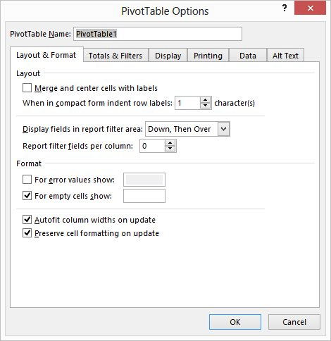
Figure 1. The Layout & Format tab of the PivotTable Options dialog box.
Now, when you refresh the PivotTable, your previously applied formatting should remain on rows and columns previously in the PivotTable. If the refresh results in new rows being added to the PivotTable, then you will still need to format those, unless you are using an AutoFormat.
ExcelTips is your source for cost-effective Microsoft Excel training. This tip (8731) applies to Microsoft Excel 2007, 2010, and 2013. You can find a version of this tip for the older menu interface of Excel here: Maintaining Formatting when Refreshing PivotTables.

Excel Smarts for Beginners! Featuring the friendly and trusted For Dummies style, this popular guide shows beginners how to get up and running with Excel while also helping more experienced users get comfortable with the newest features. Check out Excel 2013 For Dummies today!
PivotTables are great for digesting and analyzing huge amounts of data. But what if you want part of that data excluded, ...
Discover MoreIf you are using a data set that includes a number of zero values, you may not want those values to appear in a ...
Discover MoreAre you attached to the classic PivotTable layout? Looking for a way to make that layout the default for new PivotTables? ...
Discover MoreFREE SERVICE: Get tips like this every week in ExcelTips, a free productivity newsletter. Enter your address and click "Subscribe."
2022-11-10 08:28:40
Sharon
Jill - Thanks for your thanks to Allen. I start every workday reading his tips. He's a rock star! I've taught Excel 1-3 at the community college and business/industry levels, and always recommended Allen's tips. I've told many of my participants, if you want a Master's Degree in Excel, here's one tool to get there. He deserves much thanks. Thanks, Allen!
2022-11-10 06:54:28
Jill
I would also recommend 'unchecking' the 'autofit column widths on update' as that can cause layouts to change significantly too! Thank you for all your tips and tricks! Excel is such a powerhouse and you help us tap into it bit by bit!
2022-02-16 18:14:23
Mark B
I found a consistently robust solution: Apply conditional formatting based on the names of the Fields used in your PivotTable. More specifically, apply Conditional Formatting for all numeric Values (columns) used in the PivotTable. I'm using PowerPivot in what I describe below.
Step 1. Click on a column with a numeric field, and apply conditional formatting based on the field, as shown in the figure. Check "All cells showing ..." The ... should show the name of the numeric Value you want to display (second button).
Step 2. Select the Rule Type "Format only cells that contain". Edit the Ruel Description to Format only cells with cell values between X and Y. Choose values for X and Y that ensure your Value field is always in that range.
Step 3. Click Format... and set up the desired numeric format as usual.
Step 4. Apply Conditional Formatting for each Value to the entire PivotTable. That way, when Value columns are moved their formatting moves with them.
(see Figure 1 below)
One more thing. I typically define "Measures" in Power Pivot for all the quantities that might appear in the PivotTable. Yes, even the "Sum of", "Count of", etc simple types of measures that don't require a formula to define. I find that helps simplify managing the tables, and drives use of consistent reporting measures across multiple pivot tables sharing the same source data.
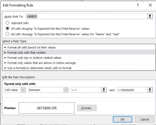
Figure 1. Apply rule to all cells showing your measure
2021-12-11 19:00:24
Chris
This doesn't work if it's a calculated field.
2021-02-01 11:57:56
Stacy S Scott
Nope doesn't work - every time I refresh the conditional formats still come off.
2020-12-31 10:15:27
Joe
This was driving me absolutely insane! I have a sheet with multiple tabs, multiple pivot tables. They all kept the borders when data was refreshed or when a slicer was used. I added 2 new pivot tables, and the borders kept disappearing. I tried everything I read online about how to fix it but every time I would refresh or select from a slicer, the borders would disappear.
THE FIX FOR ME:
I saved the file, closed excel, and reopened it. When I did that, the borders stayed on the new pivot tables with no issue. Not sure why that happened but it caused me about a half hour of yelling at my screen before I tried it!
2020-07-21 17:53:41
David
Problem seems to occur when using the Format Painter to copy formats from one pivot table to another. I had a worksheet in a file with several pivot tables, and after using the format painter to help format fonts and fills, I found the same problem when refreshing the file: formats would be lost, even though the preserve formatting box was checked in the Pivot Table Options.
I then deleted all the formatting from all the tables, and removed all filters from the tables, and started formatting each table individually.
When finished, the formatting stayed in place after a Refresh All. I then reapplied the filters I wanted, refreshed again, and the formatting still remained.
2020-03-10 21:51:23
Nico
You will need to use set the number format in Value Field Settings first, then on "Refresh" the number format will always revert to the defined format
(see Figure 1 below)
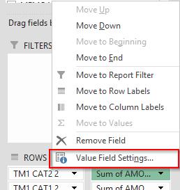
Figure 1.
2019-10-22 16:15:36
cS
And how do you troubleshoot when that box IS checked but the formatting is NOT being preserved!??
2019-07-22 18:11:46
richard becraft
Does not work on Excel 2016 pivot table with conditional formatting.
2019-04-29 17:36:47
OD
The thing that worked for me was removing my label filter removing the (blank) label and instead apply a value filter to remove the row with a 0 value--which thankfully was my (blank) row. For whatever reason switching from one type of filter to the other worked for retaining font size. And the result is the same whether I filter for (blank) or 0. Thank God for a solution. This was painful.
2019-04-24 04:43:36
Olly J
Where it comes to column header format refreshing despite the option to no reformat being selected (!), I found that if you first apply a format pre-set within excel e.g. "Normal 3" and then reapply your formatting; it will successfully allow the formatting to stick.
2019-02-17 02:31:55
Tom
This does not work for 2010
2019-02-16 10:54:05
Ken Cameron
Allen, I have O365. Do you have or could you research any updates on this issue? I religiously do the tasks in your tip, but Excel still randomly and selectively wipes out my pivot table formating.
2018-12-28 16:32:51
jeff kidd
Does not work when using "Conditional Formatting".
2018-11-30 16:19:24
no
Good job at creating a guide that doesn't actually apply to anything. These options are on by default and they don't change anything. Refreshing the table still removes all conditional formatting.
2018-10-09 08:05:10
Paresh Patel
I have performed this task as described to retain the formatting on a pivot table but when i refresh some of the formatting reverts back to the original formatting. any ideas I am using Excel 2013.
Any help would be appreciated as I update the main table and have created a summary table via a Pivot table which I present to the client on a weekly bases
2018-09-22 01:20:59
Maintaining Formatting when Refreshing PivotTables
by Allen Wyatt
(last updated August 25, 2017)
This does not work for Excel 2010. Wish I could find something that does!
Particularly cell border formatting but other formatting also.
2018-08-14 12:06:25
CS
When i did this, step by step, everything in my pivot table went o centered alignment.
2018-06-15 06:58:38
Paul
Reviewed and tried all of these comments - didn't work for me.
My pivot table has a slicer and every time I selected a filter or refreshed the pivot table, all formatting was lost. I my case a specific column was formatted as number with no decimals, when refreshed certain cells changed to general format.
Then playing around I found if I selected the entire sheet, (triangle top left hand side between Col A and Row 1) and then formatted all data right using the alignment icon at the top of the page all worked ok for me.
Hope this helps
2018-05-30 14:23:40
shilpa567@gmail.com
Right click on Pivot table->Pivot table Options ->Preserve cell formatting on update doesn't seem to effect much when used slicers.
Try this method:
First Select the values you want to format or click anything on the slicer->Now Go to Conditional Formatting->New Rule or Manage Rules->It opens up the window as
New/Edit Formatting Rule dialog window:
Apply rule to :
1)Selected cells
2)All cells showing “Field” (Use this)
3)All cells showing “Field values” with ……
Now select your condition
For ex: Format only cells that contain less than or equal to “2” Format to Yellow.
Format only cells that contain less than or equal to "3" Format to Orange.
The slicer format will still remain because you have selected Field instead of selected values.
*If you want to add more conditions simply follow the above and create new rule.
(see Figure 1 below)
(see Figure 2 below)
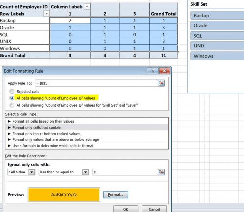
Figure 1. Conditional Formatting for Pivot Table with slicers
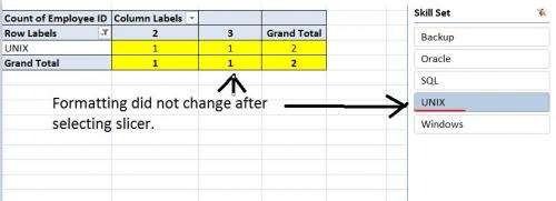
Figure 2. Format doesnt change now even after selecting the Slicer
2018-03-08 15:46:43
Johnny A.
For conditional formatting issues this worked for me in Excel 2010: Select a cell in the column you want to show conditional formatting and select "New Rule" then you should get several buttons. Select the one that says "All Cells Showing Values". Unfortunately you have to do if for each column. When I refresh or use filters, my conditional formatting stays intact.
Hope this helps!
2017-12-11 10:32:22
Stephanie Johns
That check box doesn't work at all.
2017-12-07 15:19:09
mel
Anne's suggestion also worked for me. I was selecting multiple tabs, CTRL-A to select everything on those tabs, and then changing fonts. The proper checkboxes (preserve cell formatting) were checked, yet that formatting would get lost every time the data was updated. Clicking the black down arrow so that specifically the pivot table was selected and THEN following those steps caused the formatting to stick as intended. Not great to do it on lots of different tabs in the same spreadsheet, but at least next time I'll know to follow those steps before I start copying and editing full sheets.
2017-10-02 13:58:51
Dru
I have a similar question to Danielle (8/24). I have pivot tables that when the data is refreshed loses the conditional formatting in the cells. I have 5 columns of data - Customer Name (L), YTD 2017 (M), YTD 2016 (N), Annual 2016 (O), Annual 2015 (P), % 17 v 16 (Q). Columns L thru P are updating each month, Column Q is a calculated field of Col M/Col N. The conditional formatting is set to change the entire line a certain color based on the % in Col Q. The conditional formatting works until the data is updated for new month. When I look at the info in the conditional formatting rule for that table (or any of them that I have) the original data range of $L$6:$Q$97 then changes to $L$6:$L$97;$Q$6:$Q$97. I have "Preserve cell formatting on update" checked in PivotTable Options. I cannot figure out how to keep the original conditional formatting rule from changing upon refresh. Any solutions?? Again - this is conditional formatting, not font, alignment, number, column width etc.
2017-08-24 08:24:56
Danielle
I have a conditional format in my pivot table for columns A through C. Columns A and B have data and Column C is the total column for the data. Although I have the conditional formula created for the range of =$A$46:$C$62, when I refresh it it changes to =$A$46:$B$62 and the total column is not formatted per the conditional formula. I have used the Options for maintain the formatting in the pivot table but nothing has worked. If anyone can provide guidance I would appreciate it. (see Figure 1 below)
Figure 1.
2017-08-05 17:56:52
Brooks
This advice doesn't disclose that only SOME formatting is preserved. For instance, if you change the borders, then refresh, MS Excel still formats borders and even worse, formats them in an inconsistent manner...
2017-05-23 05:05:24
Timothy Joy
That solution didn't work for me.
The tips that did work are:
1. take off any filters you have in the pivot table. (<<< THIS WAS KEY)
2. hover the point over the header until it forms a black down arrow to select the entire column (or over the row header left edge, to select a row)
3. tick "preserve formatting on update" in the p-t option (although this is seems to be not meaningful)
Tim
PS: Credit where credit is due, my solution comes from http://datapigtechnologies.com/blog/...omment-1492670
2017-05-04 13:56:28
Marc Hawk
ANSWER!!!!
When using a slicer, select all options. Format properly, then when you select a subset of the larger table using the slicer. It will be formatted properly. If you only format on the subsection of your pivot table. It will look odd when you choose another subset of the data.
preserve formatting should be checked.
2017-01-31 09:46:45
Alan Jones
Didn't work completely. Some remained...some didn't! On refresh, it seems that cells (randomly it seems) 'forgot' that they were centred in the cell...and borders (randomly it seems) disappeared.
Any ideas??
2017-01-24 09:29:21
Arnold
Try to click on each cell in a column randomly...you will come to a point where all cells will suddenly be highlighted...that will be the time you can right click and format cells...after you do this...try to refresh..you will see that all cell in that column has retained its formatted values...Enjoy Everyone...
2016-11-09 17:50:48
Lauren
Still lose formatting when pivot is refreshed.
2016-08-26 14:10:18
Chris M
I'm with Trisha.
Pivots simply cannot retain the formatting. Examples: Fonts and Alignments.
2016-08-18 19:17:42
JA
Hi. A few weeks ago, the company, upgraded Windows (not exactly sure how) and it affected my ability to retain pivot formatting in Excel 2013. I have one file that will retain the format when new data has been added to the range and two other files were I continually have to reformat (e.g. Add borders, shading, bold/underline, etc). I've read through the comments starting with this string and still don't seem to have a proper solution. I made sure the "Preserve cell formatting on update" has been checked. The file that retains was saved with an Excel Worksheet extension vs Excel 97-2003 Worksheet. Tried to change the extension and no luck. Last resort is to include IT, but this is a weird fluke after some kind of add-ins were done.
2016-08-13 07:05:09
jd murphy
Thanks Jim Swindle. My query isn't related to Pivot Tables so maybe I'm intruding into the wrong forum. Just in a general Excel sheet I find it a great inconvenience when I 'Replace All' I have to go back and re-italicize where necessary. There are 154,000 rows x 10 cells in the file.
I'll try to keep out of jail.
2016-08-12 07:00:12
Jim Swindle
jd murphy, if you're using Find and Replace on a PivotTable, there's something odd about your process. A PivotTable is linked to source data. If you change the result data manually, that probably means either that there is something wrong with the source data (which should be fixed) or that you're adjusting the results in ways that they should not be adjusted. Of course, maybe you're just adjusting the spelling of a label that some bureaucracy won't let you fix in the source, but again, you or your organization may have a bigger problem than Excel. I'm cautious, because years ago I innocently helped a likable guy modify data; it turned out that he was hiding risk. When it was discovered, he went to prison.
2016-08-12 05:56:53
jd murphy
Find and Replace loses all type formatting. Specifically italics disappear. Help!
2016-08-11 09:03:08
I have worked with Pivot Tables for years. I always check the two boxes needed to keep the formatting and the column widths. I also know to format the columns, you do it from the table itself with the little black arrow instead of the Excel column letters on top... it still doesnt work. I was told this is an Excel glitch that has happened for years. I thought that maybe every time they come up with a new version, they would fix these issues but I guess they didnt. UGH... How frustrating.
2016-07-06 05:44:37
Donat Protzen
Hello,
The layout of the columns is not yet fixed unless the box "Autofit column widths on update" is unchecked.
This helped me get the format to stick.
2016-05-16 12:47:59
Amy Laughlin
Hello,
I am drawing numbers from another excel sheet and they appear in the pivot but not in order. I have checked formatting for both and ensured they are the same but there are five numbers that will not sort in order?
Can you assist please?
2016-03-01 05:49:00
Ben
Thanks for this, Dan. However, this doesn't appear to work on Data Labels in a Pivot Chart.
I'm using Excel 2010 and to suppress zero values on the Pivot Chart data labels, I've formatted them to #,###;;;
When I check the preserve formatting box in the source pivot table and then refresh the table, the formatting disappears. Any ideas on how to prevent this? The only solution I've found involves a macro.
Ben.
2016-02-24 16:53:00
AC2
THANK YOU DAN! (Feb 28 commenter)
2016-01-26 13:57:51
Daniel
Well, that was easy! Thanks!
2016-01-25 16:49:08
Mike
Things were dire. We needed a hero. And so Anne appeared, dropped a knowledge bomb, and walked away from the explosion without even flinching. Her contribution has transcended space, time, newer additions of Excel, and the uselessness of this article. We salute you, Anne. We will go forth and spread tales of your bravery throughout the land.
2016-01-07 12:59:45
Michael Kelley
This did not work for conditional formatting for me. I wanted every other row to be shaded gray, and when I would click on the little + or – to expand or collapse the information the shading would go away. One thing I noticed is the shading will go away on the values part but not on the rows part. To get it to stay you must conditional format each part of the pivot table separately, one conditional rule for the rows section (the labels on the left) and one for the values section (on the right). When I did that the shading stayed.
2015-12-14 15:17:18
Patty
I am confused as I do not have an option tab in Excel 2013, so I can go no further than this step.
4.Display the Options tab of the ribbon.
My actual problem is, when I refresh the data, my "Row Labels" disappear.
2015-12-03 04:13:06
Abhijit Ghosh
For those who dont find that black pointer while moving over pivot. You can go to Analyze on the Pivot tables tool and under actions you will find the magic wand. There are options to select enable selection. Explore that more. you will find the solution as i did.
2015-11-12 08:53:01
Greg van Staden
I find none of these work effectively. What does work and thank you to my brother, change all the formats you want including column widths.
Highlight all the columns and Group together. (I normally leave first column visible)
Before refreshing the Pivot, collapse the columns, after pivot refresh expand thecolumns and you will find all column widths and formats have remained the same and the data has refreshed (UIDUIW)
2015-11-07 04:02:49
James Knight
Thanks for the tip
simple fix to an annoying problem.
All I need now is a fix to getting the data and filling the damned thing!!
2015-10-07 11:01:54
Richard
I'm sorry, but saying to individually select cells, or clicking on preserving cell formats, is redundant, and incredibly unhelpful since IT CLEARLY DOES NOT WORK
2015-08-27 11:18:30
AC
On Excel 2007 I have much better luck when I set the formatting before adding any pivot table filters. If you are still having issues after these tips try removing all filters - set the formatting and check the box to preserve - then add the filters back at the end.
2015-06-19 16:14:45
Jim Swindle
CORRECTION to what I'd just posted...
In summary, it looks like there are two things to do to get Excel to keep number formats in a PivotTable:
First, right-click in the PivotTable and in PivotTable Options select "Preserve cell formatting on update."
Second, click on the field name cell in the top row of the table (NOT on the Excel column header). Hover over the top edge of the cell until you can click the black arrow, then right-click and choose "Number format." Format as needed.
2015-06-19 16:08:29
Jim Swindle
Thanks! In summary, it looks like there are two things to do to get Excel to keep number formats in a PivotTable:
First, right-click in the PivotTable and in PivotTable Options select "Preserve cell formatting on update."
Second, hover over the top of the field name cell in the first row of the table (NOT on the Excel column header) until you can click the black arrow, then right-click and choose "Number format." Format as needed.
2015-06-04 09:48:09
Diane
Regarding Anne's solution: I do not get a tiny black arrow when I hover on the column title. I only get a down-pointing black arrow when I hover on the column header (the letter of the column). I would like one column in my pivot table to always be centered text. When I close and reopen, some of the rows are centered and some are not. Is there a way, once and for all, to to have formatting permanently maintained?
2015-05-28 02:50:24
maija
for some reason when i do this my pivot does exactly opposite, it loses my formating for a part of pivot table which is very strange, cannot understand why. at the same time another pivot table at the same sheet works fine
2015-04-29 04:55:21
tristan
Good Day,
Guys need your help regarding my pivot conditional formatting. For example I have a source data with list of accounts that have status for example of, penetrated, no potential, new account etc. How can i color code my pivot cell per account based on their account status on source data?
2015-04-23 11:41:01
Dale
Dan's comment on Feb 28 was very helpful for me. Each header cell needs to be separately formatted in order for it to stick when expanding or collapsing rows.
2015-03-31 15:36:25
Gary
Dan: Thanks for the post 28 Feb 2015, 14:56! I've been trying to figure this out for a long time.
Allen:
Thanks for your Excel and Word tips. Great resource!
2015-03-16 09:49:15
Dave
Good job Anne.... Exactly my problem!
2015-02-28 15:01:22
Dan
In addition to my previous post... I should clarify that you'll still need to have the "Preserve cell formatting on update" option turned on, I also have the "Autofit column widths on update" turned OFF. Also; using Office 2013.
Happy Excelling!
2015-02-28 14:56:04
Dan
Sorry if this is redundant (if I missed it in another comment).
After trying many of the suggested approaches I was still unable to keep the formatting in my Header Row (as using slicers/filtering. The fix that worked for me: Individually select each header in the pivot table, Right-Click "Format Cells...", then specify my format options. I tried it a couple ways (both worked): Simply select the cell, right-click... Or, wait for the black column select arrow to appear, then right-click cell (again both worked).
I posted this in case someone else was about to loose their mind (like I almost did - kidding of course).
2015-02-20 15:14:44
MGG
The tip with the black arrow does allow formating of the whole column or row, but what if I want o have the formating done only to the column headers ?
2015-01-29 23:33:37
I would like to seek help on how to maintain value field settings in MS Excel 2010 when pivot table are being refreshed.
I have a pivot table where one column has a value field setting of (% Running Total). Every time I open the said saved excel sheet and refresh it, the value field setting on the said column is changing to "No Calculation."
2015-01-22 07:45:35
brian Murray
Anne 07 Oct 2013, 10:57 solution is the only one that worked for me.. thank you anne
where ever you may be :)
The correct procedure is to hover on the column title within the pivot table until the tiny black arrow appears, then click in the column. This will only allow the selection of data within the table itself, not above or below it.
2015-01-07 11:31:01
Martin
Thank you to Anne for solving a problem that has bugged me for ages.
2014-12-31 11:29:39
Oscar
SOLUTION - I would format Column F by selecting the column header, and change the number format to currency. It worked but only for an instance. It kept defaulting to General every time I would refresh. I read Anne's posting and it only made sense so I decide to try. I simply selected a cell within the pivot table of the column I wanted to format, changed it from general to currency, and it worked like a charm. Doesn't change when I refresh or when I open the file. Thank you, Anne. I think you solved the mystery for many of us.
2014-12-16 13:34:46
Hal
This does NOT reliably work.
2014-11-01 08:25:27
Narendra chouhan
a lot lot lot lot lot lot lot lot lot lot lot lot lot lot lot lot lot lot lot lot lot lot lot lot lot lot lot lot lot lot lots of thanks for this tips... thank you so much....
2014-10-15 16:39:35
Francis Moore
I followed Anne's suggestion and now have a happy pivot table which does not change when I refresh the data - thank you!
2014-10-06 15:11:47
Rich
I have the exact same problem as 'Laurel', a problem with the cells going black. I have seen that it is the fill color changes. Laurel's happens in 2013 version, mine happens in 2010 version. When I select a report filter, the result is presented in 'black fill', which I can change, but who wants to do that everytime? Plus I send this report out to several others, since it is rather comprehensive w/o using the filter, no one had advised me until recently of the problem, as no one had used a filter. I inherited this particular file, and had not previously 'tested it' myself, as no one had mentioned until now. I do not know how they survived for a year without anyone utilizing in that way. I see it as a blatant (blatant) Excel glitch, but appreciate anyone's advice.
2014-08-07 15:52:01
Laural
I'm using Excel 2013, and my pivot table options are defaulted to the setting above, however I still get formatting problems when I refresh - but only on some pivot tables. Any changes cause some of the cells in the pivot table to be blacked out completely (fill color black).
I have a lot of manual color assignments to different cells to help me tie out values to another report (if that makes a difference).
2013-10-07 10:57:32
Anne
I've had the same problem as Robert. After some tinkering, I've figured out the solution.
The problem occurs when you don't select the area or areas to format correctly. For instance, when I wanted to format a column of data in a pivot table, I selected the full column as I would normally do in a regular spreadsheet. That is, I clicked on the column heading, which would be the letter name on the spreadsheet grid, so that I am including data above and below the table.
The correct procedure is to hover on the column title within the pivot table until the tiny black arrow appears, then click in the column. This will only allow the selection of data within the table itself, not above or below it.
I think doing it the other way must indicate to excel that you are formatting the area surrounding the pivot table, not the table itself, and in actuality, you are only temporarily formatting the table.
The same goes for a row.
2013-09-30 09:17:20
KD
Jan, simply deselect the autofit column widths on update' box found directly above the 'preserve cell formatting' box.
2013-09-30 08:42:13
Jan
I use Excel 2007. While the table does retain colors and fonts, it will not keep wrapped headers or column widths. Extremely frustrating.
2013-09-30 05:27:47
Duncan
I have to say that losing formatting is one of the chief reasons I dislike PivotTables.
2013-09-28 07:06:24
Robert
Excellent Excel Tip.
The problem is that this approach does not always ensure that data remains formatted within a pivot table. Furthermore, data that changes or is modified at the source can create additional issues. I had to create a Macro to delete line items that are no longer present or have been modified in the source data. I would very much appreciate if Microsoft addressed these issues once and for all.
P.S. Currently using Excel 2010.
Got a version of Excel that uses the ribbon interface (Excel 2007 or later)? This site is for you! If you use an earlier version of Excel, visit our ExcelTips site focusing on the menu interface.
FREE SERVICE: Get tips like this every week in ExcelTips, a free productivity newsletter. Enter your address and click "Subscribe."
Copyright © 2024 Sharon Parq Associates, Inc.
 Please Note:
This article is written for users of the following Microsoft Excel versions: 2007, 2010, and 2013. If you are using an earlier version (Excel 2003 or earlier), this tip may not work for you. For a version of this tip written specifically for earlier versions of Excel, click here:
Please Note:
This article is written for users of the following Microsoft Excel versions: 2007, 2010, and 2013. If you are using an earlier version (Excel 2003 or earlier), this tip may not work for you. For a version of this tip written specifically for earlier versions of Excel, click here:
Comments