Getting Rid of Leading Zeros in a Number Format

When you enter a numeric value into a cell, by default Excel will display a leading zero on values that are less than 1. For instance, if you enter the value 1.234 into a cell, Excel displays just that: 1.234. If you enter .234 into the same cell, Excel includes the leading zero: 0.234.

If you want to get rid of the leading zeros, then you need to rely upon a custom format. This is rather easy to create; just follow these steps:

1. Select the cell (or cells) that you want to format.
2. Display the Home tab of the ribbon.
3. Click the small icon at the bottom-right of the Number group. Excel displays the Format Cells dialog box.
4. If the Number tab is not displayed, select it.
5. In the Category list, choose Custom. The dialog box changes so you can enter a custom format. (See Figure 1.)



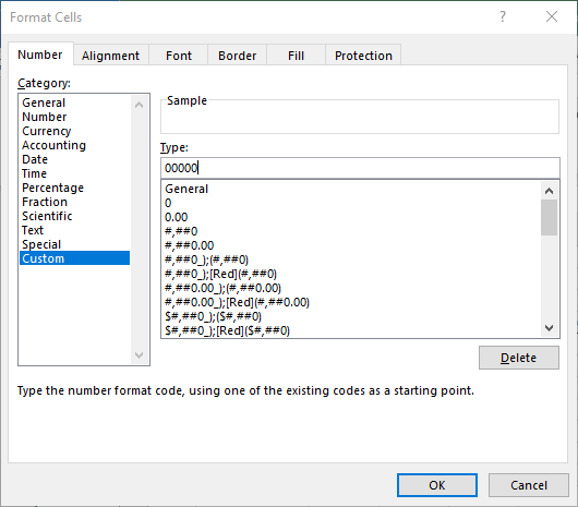
Figure 1. The Number tab of the Format Cells dialog box.

6. In the Type box, enter the following pattern: .###
7. Click OK.

That's it; the number in the cell will no longer have a leading zero if it is less than 1. There are some caveats to this, however. First, if the number you enter in the cell has more than three digits after the decimal place, then the number will be rounded (for display purposes) to only three digits. If you are going to routinely have more than three digits in the value, you should increase the number of hash marks (#) in the custom format.

Second, if the value you enter into the cell has fewer than three digits to the right of the decimal place, then only the number of digits required will be displayed. Thus, if you have multiple cells formatted this way, it is very possible for the numbers to not "line up" along the decimal point. The solution to this is to change the format to something that will always display the same number of digits after the decimal point. A good choice is, in step 6, use the format ".000" (without the quote marks). This format will always display three digits after the decimal point, adding zeros to the end of the value, if necessary.

You could also change the format a bit if you want things to line up on the decimal point, but you don't want any trailing zeros. Try replacing the hash marks (#) in the custom format in step 6 with question marks. Thus, you would use ".???" instead of ".###". This results in up to three digits being displayed, but if there are fewer than three digits the remaining question marks are replaced with spaces.

Third, if the value you enter into the cell is a whole number, then it will always be displayed with a decimal point. Thus, entering 3 in the cell results in the display of 3., with the decimal point. For most people this won't be a big deal, and there is no easy way to modify the custom format to remove the decimal point from whole numbers.

Fourth, if you enter 0 in the cell, it won't be displayed at all. Instead you get a single decimal point in the cell and nothing else. The way around this problem is to make your custom format just a bit more complex. In step 6, above, enter the following as the custom format:

[=0]0;[<1].000;General

This custom format indicates that a 0 value should be shown as 0, any value less than 1 should be shown with no leading zero and three digits to the right of the decimal point, and anything else should be displayed using the General format.

One final note: If you still see leading zeros before a number, it could be that Excel doesn't think it is a number at all. It could be that your number has been formatted as text by Excel. If you think this might be the case, click in the cell and you will see a small information icon to the left or right of the cell. Click the icon and choose the Convert to Number option from the choices presented.

ExcelTips is your source for cost-effective Microsoft Excel training. This tip (10031) applies to Microsoft Excel 2007, 2010, 2013, 2016, 2019, and Excel in Microsoft 365. You can find a version of this tip for the older menu interface of Excel here: Getting Rid of Leading Zeros in a Number Format.