Non-adjusting References in Formulas

Everybody knows you can enter a formula in Excel. (What would a spreadsheet be without formulas, after all?) If you use address references in a formula, those references are automatically updated if you insert or delete cells, rows, or columns and those changes affect the address reference in some way. Consider, for example, the following simple formula:

=IF(A7=B7,"YES","NO")

If you insert a cell above B7, then the formula is automatically adjusted by Excel so that it appears like this:

=IF(A7=B8,"YES","NO")

What if you don't want Excel to adjust the formula, however? You might try adding some dollar signs to the address, but this only affects addresses in formulas that are later copied; it doesn't affect the formula itself if you insert or delete cells that affect the formula.

The best way to make the formula references "non-adjusting" is to modify the formula itself to use different worksheet functions. For instance, you could use this formula in cell C7:

=IF(INDIRECT("A"&ROW(C7))=INDIRECT("B"&ROW(C7)),"YES","NO")

This formula constructs an address based on whatever cell the formula appears in. The ROW function returns the row number of the cell (C7 in this case, so the returned value is 7) and then the INDIRECT function is used to reference the constructed address, such as A7 and B7. If you insert (or delete) cells above A7 or B7, the reference in cell C7 is not disturbed, as it just blithely constructs a brand new address.

Another approach is to use the OFFSET function to construct a similar type of reference:

=IF(OFFSET($A$1,ROW()-1,0)=OFFSET($B$1,ROW()-1,0),"YES","NO")

This formula simply looks at where it is (in column C) and compares the values in the cells that are to its left. This formula is similarly undisturbed if you happen to insert or delete cells in either column A or B.

A final approach (and perhaps the slickest one) is to use named formulas. This is a feature of Excel's naming capabilities that is rarely used by most people. Follow these steps:

1. Select cell C2.
2. Display the Formulas tab of the ribbon.
3. In the Defined Names group click the Define Name tool. Excel displays the New Name dialog box. (See Figure 1.)



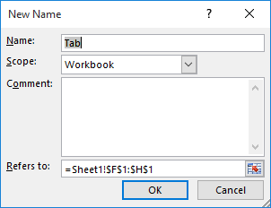
Figure 1. The New Name dialog box.

4. In the Name box enter the name CompareMe. (You can use a different name, if you desire.)
5. Erase whatever is in the Refers To box, replacing it with the following formula:

     =IF(A2=B2,"YES","NO")

6. Click OK.

At this point you've created your named formula. You can now use it in any cell in column C in this manner:

=CompareMe

It compares whatever is in the two cells to its left, just as your original formula was designed to do. Better still, the formula is not automatically adjusted as you insert or delete cells.

ExcelTips is your source for cost-effective Microsoft Excel training. This tip (12348) applies to Microsoft Excel 2007, 2010, 2013, 2016, 2019, Excel in Microsoft 365, and 2021. You can find a version of this tip for the older menu interface of Excel here: Non-adjusting References in Formulas.