PivotTable Aggregating Incorrect Data

Liesie has a PivotTable that she's been working with for some time. It is suddenly and unexpectedly pulling the wrong info from the source data. Out of 16 unique identifiers, NR22229 and NR22447 are pulling through as NR21219 and NR21447, while all the rest are correct! Liesie has checked and there is not an incorrect entry in the PivotTable data source range. She wonders what would cause the PivotTable to do this and if there is a way to correct it.

These types of issues are notoriously difficult to troubleshoot without actually working with the workbook. Even so, a few things can be suggested to fix the problem. Assuming that the identifiers are being shown in rows, it is possible that there was an inadvertent typeover of the two Row Labels (NR22229 and NR22447) in the PivotTable. The typeover would result in the data being pulled from the wrong location—whatever was typed into the Row Label area becomes the new label for that value.

If you suspect this is the issue, you can remove the identifiers field from the Field area, and then refresh the PivotTable. (Refreshing is important as it forces a renewed fetching of the data to be aggregated in the PivotTable.) You can then place the identifiers field back into the PivotTable.

If that doesn't fix the issue, then it could be that Excel is still confused on how to pull the proper data into the PivotTable. This can be especially true if you have deleted data, columns, or rows in the source data. To fix this potential issue, follow these general steps:

1. Right-click a cell within the problem PivotTable. Excel displays a list of options.
2. Choose PivotTable Options. Excel displays the PivotTable Options dialog box.
3. Make sure the Data tab is displayed. (See Figure 1.)



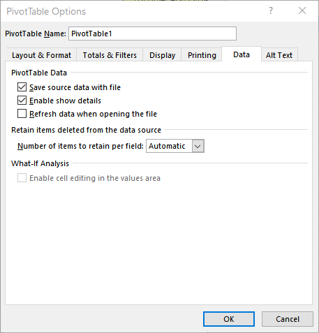
Figure 1. The Data tab of the PivotTable Options dialog box.

4. Using the Number of Items to Retain Per Field drop-down list, choose the None option.
5. Click OK.
6. Refresh the PivotTable.

If that still does not work, then the remaining (and most drastic) solution is to delete the PivotTable and recreate it from your source data.

ExcelTips is your source for cost-effective Microsoft Excel training. This tip (12882) applies to Microsoft Excel 2007, 2010, 2013, 2016, 2019, Excel in Microsoft 365, and 2021.