Please Note: This article is written for users of the following Microsoft Excel versions: 2007, 2010, 2013, 2016, 2019, Excel in Microsoft 365, and 2021. If you are using an earlier version (Excel 2003 or earlier), this tip may not work for you. For a version of this tip written specifically for earlier versions of Excel, click here: Returning Item Codes Instead of Item Names.
Written by Allen Wyatt (last updated April 27, 2024)
This tip applies to Excel 2007, 2010, 2013, 2016, 2019, Excel in Microsoft 365, and 2021
Alan can use data validation to create a drop-down list of valid choices for a cell. However, what he actually needs is more complex. He has a large number of item names with associated item codes. In cell B2 he can create a data validation list that shows all the item names (agitator, motor, pump, tank, etc.). The user can then choose one of these. When he references cell B2 elsewhere, however, he wants the item code—not the item name—returned by the reference. Thus, the reference would return A, M, P, TK, etc. instead of agitator, motor, pump, tank, etc.
There is no direct way to do this in Excel. The reason is because data validation lists are set up to include only a single-dimensional list of items. This makes it easy for the list to contain your item names. However, you can expand how you use the data validation list a bit to get what you want. Follow these steps:
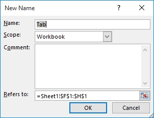
Figure 1. The New Name dialog box.
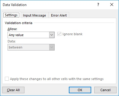
Figure 2. The Data Validation dialog box.
With these steps done, people can still use the data validation drop-down list to select valid item names. What you now need to do is reference the item code from the data table you set up in step 1. You can do that with a formula such as this:
=VLOOKUP(B2,OFFSET(Itemlist,0,0,,2),2,FALSE)
This formula can be used on its own (to put the desired item code into a cell) or it could be used within a larger formula, anyplace you would have originally referenced B2.
If, for some reason, you cannot create a data table for your item names and codes, you could approach the problem by entering your names and codes directly into a formula. Either of the following will work:
=CHOOSE(MATCH(B2,{"agitator","motor","pump","tank"}),"A","M","P","TK")
=INDEX({"A","M","P","TK"},MATCH(B2,{"agitator","motor","pump","tank"},0))
These formulas work just fine in Excel 2021 or the Excel in Microsoft 365. In other versions of Excel you'll need to enter it as an array formula by pressing Ctrl+Shift+Enter.
The biggest drawback to the in-a-formula approach is that it can quickly become unwieldy to keep the formula updated and there is a "viability limit" on how many pairs of codes and items you can include in the formula. (The limit is defined by formula length, so it depends on the length of your item names.) Also, this approach is good to only return the item code in another cell, rather than including it as part of a larger formula.
ExcelTips is your source for cost-effective Microsoft Excel training. This tip (12078) applies to Microsoft Excel 2007, 2010, 2013, 2016, 2019, Excel in Microsoft 365, and 2021. You can find a version of this tip for the older menu interface of Excel here: Returning Item Codes Instead of Item Names.

Excel Smarts for Beginners! Featuring the friendly and trusted For Dummies style, this popular guide shows beginners how to get up and running with Excel while also helping more experienced users get comfortable with the newest features. Check out Excel 2013 For Dummies today!
Excel allows you to easily develop formulas that pull values from worksheets and workbooks other than the one in which ...
Discover MoreYou can use the CLEAN worksheet function to remove any non-printable characters from a cell. This can come in handy when ...
Discover MoreExcel allows you to easily convert values from decimal to other numbering systems, such as hexadecimal. This tip explains ...
Discover MoreFREE SERVICE: Get tips like this every week in ExcelTips, a free productivity newsletter. Enter your address and click "Subscribe."
2024-04-27 11:15:37
J. Woolley
In step 1 of the Tip, a table is defined with two columns (item names and item codes). Later in the Tip is the following formula:
=VLOOKUP(B2,OFFSET(Itemlist,0,0,,2),2,FALSE)
The Tip forgot to mention the table in step 1 must be named Itemlist. Select the table, then pick Table Design > Properties > Table Name (Alt+JT+A).
Got a version of Excel that uses the ribbon interface (Excel 2007 or later)? This site is for you! If you use an earlier version of Excel, visit our ExcelTips site focusing on the menu interface.
FREE SERVICE: Get tips like this every week in ExcelTips, a free productivity newsletter. Enter your address and click "Subscribe."
Copyright © 2024 Sharon Parq Associates, Inc.
 Please Note:
This article is written for users of the following Microsoft Excel versions: 2007, 2010, 2013, 2016, 2019, Excel in Microsoft 365, and 2021. If you are using an earlier version (Excel 2003 or earlier), this tip may not work for you. For a version of this tip written specifically for earlier versions of Excel, click here:
Please Note:
This article is written for users of the following Microsoft Excel versions: 2007, 2010, 2013, 2016, 2019, Excel in Microsoft 365, and 2021. If you are using an earlier version (Excel 2003 or earlier), this tip may not work for you. For a version of this tip written specifically for earlier versions of Excel, click here:
Comments