Written by Allen Wyatt (last updated March 12, 2025)
This tip applies to Excel 2007, 2010, 2013, and 2016
Marcya has a long list of sorted numbers in column A of a worksheet. These numbers are supposedly consecutive, but she doesn't know if that is true. Examining the list manually is both tedious and error-prone, so Marcya wonders if there is a way to somehow highlight any "missed numbers" (those that aren't consecutive with the one before) or to compile a list of numbers that were missed in the list.
There are a number of ways you can go about figuring out where there are missing numbers. The first is one I use quite often: I add a helper column next to column A. Assuming your numbers start in cell A1, I put this into cell B2:
=IF(A2<>A1+1,"Error","")
Copy the formula down as many cells as necessary, and you'll easily see the word "Error" next to any value that isn't consecutive to the value just above it. If you prefer to know a bit more about the error, you could use a more detailed formula:
=IF(A2=A1,"Duplicate",IF(A2<>A1+1,"Gap",""))
Another approach is to use conditional formatting on the cells in column A. Follow these steps, again assuming that your values start in cell A1:
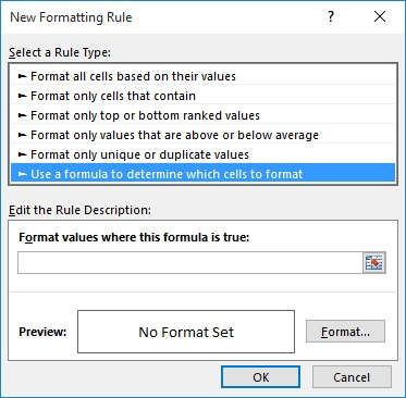
Figure 1. The New Formatting Rule dialog box.
Finally, if you want to compile a list of the missing numbers in a consecutive series, you can use an array formula. Place the following into row 1 of an empty column:
=IFERROR(SMALL(IF(COUNTIF($A$1:$A$135,
MIN($A$1:$A$135)+ROW($1:$135)-1)=0,
MIN($A$1:$A$135)+ROW($1:$135)-1),ROW(A1)),"")
Remember that this is a single array formula, so you need to enter it as a single line using Ctrl+Shift+Enter. You can then copy the formula down a number of cells, until it doesn't return any more values. Also, the formula assumes that your series in in the range A1:A135; if it is not, you'll need to modify the formula to reflect the actual range.
ExcelTips is your source for cost-effective Microsoft Excel training. This tip (4315) applies to Microsoft Excel 2007, 2010, 2013, and 2016.

Excel Smarts for Beginners! Featuring the friendly and trusted For Dummies style, this popular guide shows beginners how to get up and running with Excel while also helping more experienced users get comfortable with the newest features. Check out Excel 2019 For Dummies today!
Excel makes it easy to concatenate (or combine) different values into a single cell. If you need to combine a different ...
Discover MoreThe formulas in your worksheet can be displayed (instead of formula results) by a simple configuration change. You can ...
Discover MoreThe precision of numeric values you display in a worksheet can be less than what is actually maintained by Excel. This ...
Discover MoreFREE SERVICE: Get tips like this every week in ExcelTips, a free productivity newsletter. Enter your address and click "Subscribe."
2023-04-12 09:18:07
Tzica
Hello, nice array formula.Somehow is limited by the missing range ? I try it on a list with 22 numbers ( a range of 13 to 74, with gaps between 14 and 25 25 to 29 / 29 to 32..an so on).Formula show missing number till 34...and than empty for the other missing number..between 37 and 53 etc..
(see Figure 1 below)
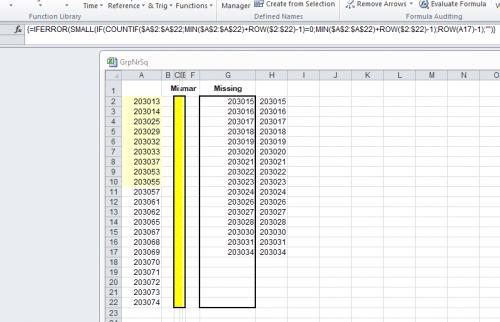
Figure 1. MissingNr
2023-02-24 10:44:19
J. Woolley
@rr1024
Addendum to my previous comment - In case the number needs to be rounded, try this:
=IF(INT(B2+1.5)=INT(B3+0.5),"True","False")
or simply this:
=(INT(B2+1.5)=INT(B3+0.5))
By the way, Microsoft does work consistently, but not always as you expected.
2023-02-23 10:04:48
J. Woolley
@rr1024
You are assuming that the "1 minute counts" have no seconds. If they are derived from date serial numbers like NOW(), then they probably do. Try this:
=IF(INT(B2+1)=INT(B3),"True","False")
2023-02-23 06:08:28
Steve J
@rr1024
as your data I get TRUE, FALSE, FALSE which is correct. You have indicated that B4 = 3 which is the same as B3.
So B3 +1 will not = B4 so will be FALSE
You don't need the =sum element in your formula, =IF(B2+1=B3,"True","False") will work perfectly.
HTH
2023-02-22 18:29:46
rr1024
I have been trying to get this to work all day long and nothing works in excel for any of the IFs I create.
I have a simple list of numbers that represent 1 minute counts, so column B starts with B2=2, B3=3, B4=3 and in column A I have, starting in A3, =IF(SUM(B2+1)=B3,"True","FALSE")
=IF(SUM(B3+1)=B4,"True","FALSE")
=IF(SUM(B4+1)=B5,"True","FALSE")
I have FALSE, FALSE, FALSE column A and I should have True, True, False
Fundamentally this is probably way so many people hate Microsoft because it just does not work consistently.
The whole column is formated for whole numbers except the top header
2022-12-01 05:32:31
Peter Atherton
Damian
The easiest way is to convert the data to a table by selecting a cell in the data and pressing Ctl + t. Table are dynamic and expand as data is added below. To convert it back to a range choose convert to range in the Tools section of the Table menu.
There is also an older method, it is not fully dynamic and it uses a couple of formulas.
=OFFSET(Sheet5!$A$2,0,0,COUNTA(Sheet5!$A$2:A500000),1)
A2 starts the range, they should alway have a Header. The two zeros refer to rows and columns to be offset, we do not want that. COunta counts the Rows with data and the range is limited to half a million to save Excel having to work too hard. The final 1 limits the range to just one column.
It is ages since I last used this method.
Peter
2022-12-01 01:06:44
Damian Barrera
I am having trouble getting the missing numbers once I expand the range. My sequence begins with the number 97680 and ends with 198698. The min number is 97680 (A1) and the max number is 198698 (A99062). So when I revise the range to read A1:A99062 it does not work. Any ideas?
2021-10-06 17:56:36
legally clueless
(see Figure 1 below) does anyone know how to identify the missing numbers if the data is listed in one column separated by a ","?
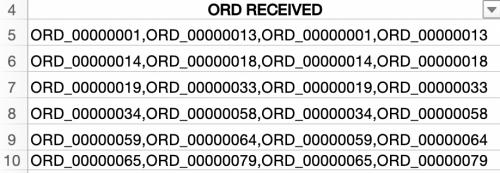
Figure 1.
2021-07-30 03:17:56
Peter Atherton
Lona
The formulas for the helper cells are:
=MIN (right(rng)+0) and
=Max(Right(range)+0)
Both are entered as Ctrl + Shift + Enter (CSE) and Excel wraps the formulas in curly brackets. In the code these are cells F3 and F4 and are the values for the variables M and N.
The last post was supposed to include a picture to make this clear, I'll try again.
(see Figure 1 below)
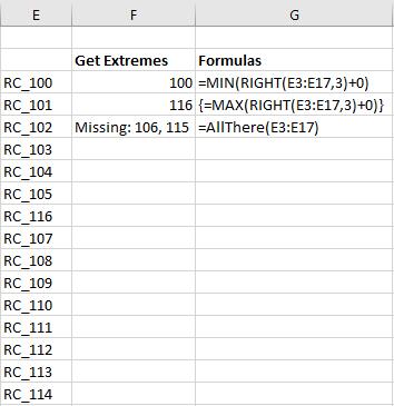
Figure 1.
2021-07-30 03:00:17
Peter Atherton
Lona,
The following needs two helper cells to get the min & max of the numbers; these are both array formulas. The code works up to numbers 999 and will need to be modified for numbers 1000 - 9999, 10000 - 99999 and so on.
Function AllThere(MyRange As Range)
Dim m As Integer, n As Integer
Dim There As Variant, i As Long, cell As Range
m = [f3]: n = [f4]
ReDim There(m To n)
On Error Resume Next
For Each cell In MyRange
There(Right(cell.Value, 3)) = 1
Next
On Error GoTo 0
AllThere = "Missing: "
For i = m To n
If Not There(i) = 1 Then
AllThere = AllThere & i & ", "
End If
Next i
If Len(AllThere) = 9 Then
AllThere = "All There"
Else
AllThere = Left(AllThere, Len(AllThere) - 2)
End If
End Function
{[fig}]
2021-07-28 11:52:03
Lona
What if my numbers start with two letters, RC_100, RC_101
2021-05-07 03:23:12
Mike
Further to my previous comment, the array formula may fail to identify some gaps.
If, for example, A1 contains 100 and the sorted list is from A1 to A135, the formula will not reveal any gaps greater than 235.
In other words, all gaps greater than (MIN(A1:A135) + 135) will be missed.
2021-05-06 11:57:11
robert Lohman
Mark
The UDF (User Defined Function) that I noted does not care about consecutive numbers. Works with any list of numbers.
2021-05-05 17:10:57
Robert Lohman
Here is a handy little Macro from Mr Excel/ExcelisFun Dueling Excel. It even lists what number(s) is missing. Just set the amount of numbers in the list. In this case it is 1 to 99
Function AllThere(MyRange As Range)
Dim There(1 To 99) As Integer
On Error Resume Next
For Each cell In MyRange
There(cell.Value) = 1
Next
On Error GoTo 0
AllThere = "Missing: "
For i = 1 To 99
If Not There(i) = 1 Then
AllThere = AllThere & i & ", "
End If
Next i
If Len(AllThere) = 9 Then
AllThere = "All There"
Else
AllThere = Left(AllThere, Len(AllThere) - 2)
End If
End Function
2021-05-05 13:44:04
Mark
Is there a way to check for missing numbers, if the list to search from is not in consecutive order?
2021-05-05 10:19:56
Mike
I don't know what I'm doing wrong but if, for example, I create a list with 10 gaps, the copied formula is only finding the first 9. The last one always seems to be missing.
2020-11-03 06:21:28
Peter Atherton
Jair
You can,, as stated in the last paragraph, copy the formula down to get the next value(s), When this is done, the Cell reference in the last part of the formula changes from Row(A1) to Row(A2) and the small value hence uses the fist then the second value.
{=IFERROR(SMALL(IF(COUNTIF($A$1:$A$135, MIN($A$1:$A$135)+ROW($1:$135)-1)=0, MIN($A$1:$A$135)+ROW($1:$135)-1),ROW(A1)),"")}
{=IFERROR(SMALL(IF(COUNTIF($A$1:$A$135, MIN($A$1:$A$135)+ROW($1:$135)-1)=0, MIN($A$1:$A$135)+ROW($1:$135)-1),ROW(A2)),"")}
2020-11-02 18:29:06
Jair
How to display all missing numbers in one column?
If i paste this formula
=IFERROR(SMALL(IF(COUNTIF($A$1:$A$135,
MIN($A$1:$A$135)+ROW($1:$135)-1)=0,
MIN($A$1:$A$135)+ROW($1:$135)-1),ROW(A1)),"")
it will apears only the first missing number how about the next missing gap?
2019-08-05 16:30:52
Gail
This is perfect! You have saved me a ton of time.
2017-09-08 10:09:56
Yvan Loranger
1st solution:
Put in B2 =IF($A2-$A1>column()-1,$A1+column()-1,"") and replicate.
Result:
row col.A col.B col.C col.D
1 -5
2 -1 -4 -3 -2
3 0
4 2 1
5 3
2nd solution:
Put in B2 =IF(A2-A1>1,A1+1&"-"&A2-1,"") and replicate.
Result:
row col.A col.B
1 -5
2 -1 -4--2
3 0
4 2 1-1
5 3
Got a version of Excel that uses the ribbon interface (Excel 2007 or later)? This site is for you! If you use an earlier version of Excel, visit our ExcelTips site focusing on the menu interface.
FREE SERVICE: Get tips like this every week in ExcelTips, a free productivity newsletter. Enter your address and click "Subscribe."
Copyright © 2026 Sharon Parq Associates, Inc.
Comments