Please Note: This article is written for users of the following Microsoft Excel versions: 2007, 2010, 2013, 2016, 2019, and 2021. If you are using an earlier version (Excel 2003 or earlier), this tip may not work for you. For a version of this tip written specifically for earlier versions of Excel, click here: Viewing More than Two Places in a Worksheet.
Written by Allen Wyatt (last updated June 26, 2025)
This tip applies to Excel 2007, 2010, 2013, 2016, 2019, and 2021
Jesse asked if there is a way to view more than two areas of a worksheet at the same time, other than by hiding rows.
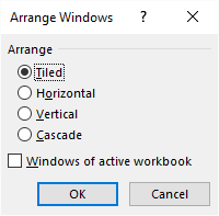
The easiest solution is to just open additional windows for the worksheet. Display the View tab of the ribbon and click New Window in the Window group. Excel opens additional windows that contain the exact same worksheet. You can then click Arrange All in the Window group of the ribbon to arrange the windows any way desired. (See Figure 1.)

Figure 1. The Arrange Windows dialog box.
When you open additional windows in this manner, the windows are independent of each other, meaning that you can scroll them independently. If you make a change in one window, the same change is made in all the windows. (This makes sense, since they all display the same data.)
Once the windows are situated the way you want them, you could save the arrangement as a view. (Display the View tab of the ribbon and, within the Workbook Views group, click Custom Views.) That way you could quickly recall the appearance of your windows any time you desire.
ExcelTips is your source for cost-effective Microsoft Excel training. This tip (9729) applies to Microsoft Excel 2007, 2010, 2013, 2016, 2019, and 2021. You can find a version of this tip for the older menu interface of Excel here: Viewing More than Two Places in a Worksheet.

Professional Development Guidance! Four world-class developers offer start-to-finish guidance for building powerful, robust, and secure applications with Excel. The authors show how to consistently make the right design decisions and make the most of Excel's powerful features. Check out Professional Excel Development today!
Hate to take your fingers off the keyboard? Here's how you can move from worksheet to worksheet without touching the mouse.
Discover MoreWhen working with multiple workbooks, you'll typically want to resize the workbook windows so you can see the data from ...
Discover MoreMoving between to adjacent worksheets is easy; Excel provides a shortcut key to do the trick. If you want to move between ...
Discover MoreFREE SERVICE: Get tips like this every week in ExcelTips, a free productivity newsletter. Enter your address and click "Subscribe."
2025-06-26 05:36:19
jamies
There is also the option of setting up a block of formulas that show the content of one set of the date in positions adjacent to the ones you are working on.
and the copy and paste special to show a live-linked "picture" as an overlaying image, having set appropriate transparency and sizing on the displayed picture.
copy the data
select the loaction for the display
select
then select the paste dropdown selection
other paste options and linkedpicture !
sometimes useful for having totaling of colums of values overlay the top section of a freeze frames section so totalling is visible without having the totals of the columns of data in the sheet within that data.
2021-11-27 15:18:22
J. Woolley
You might also consider Freeze Panes from the Ribbon's View tab or Excel's Camera Tool. For more about the Camera Tool, see these articles:
https://excelchamps.com/blog/camera-tool/
https://trumpexcel.com/excel-camera-tool/
https://excelribbon.tips.net/T010521_Using_the_Camera_in_VBA
My Excel Toolbox includes the DynamicImage macro, which is similar to the Camera Tool or Home > Paste > Linked Picture. The DynamicImage macro copies a range of cells and pastes it as a dynamic image in any sheet of any workbook. In addition to cell values, the dynamic image will include visible portions of shapes or charts from the copied range. Any changes visible in the copied range will be reproduced in the dynamic image. The result is a simple dashboard.
See https://sites.google.com/view/MyExcelToolbox/
Got a version of Excel that uses the ribbon interface (Excel 2007 or later)? This site is for you! If you use an earlier version of Excel, visit our ExcelTips site focusing on the menu interface.
FREE SERVICE: Get tips like this every week in ExcelTips, a free productivity newsletter. Enter your address and click "Subscribe."
Copyright © 2026 Sharon Parq Associates, Inc.
Comments