Arvid notes that in older versions of Excel he was able to freeze both a row and a column by selecting a cell at the required intersection. Once done, the left and top portions of the worksheet would remain visible when scrolling. Now Arvid can only find the option to freeze either a row or a column, but not both. He wonders if he is missing something.
Somewhere over the past few versions of Excel, Microsoft changed how you freeze both columns and rows. Actually, they didn't change how you freeze them; they changed how the freezing is displayed in the various options available from the ribbon. Here's how you go about it.
First, select a cell below which you want the rows frozen and to the right of which you want the columns frozen. For instance, if you want to freeze the first 2 rows and leftmost column, choose cell B3.
Now display the View tab of the ribbon and click the Freeze Panes tool. Excel displays some options that you can choose from. (See Figure 1.)

Figure 1. The Freeze Pane Options
It is the very first option—Freeze Panes—that you want to select. If you select either of the other two, then you'll only freeze either the rows above or columns to the left of the select cell.
There is a caveat here, and it could be the cause of the confusion for Arvid. When you click the Freeze Panes tool, what you then see may not match what is shown in the previous figure. It is very possible that the first option will not be Freeze Panes but will instead be Unfreeze Panes. This is the case if there are already frozen panes in the worksheet. (In other words, someone previously chose any of the three options available through the Freeze Panes tool.) Microsoft refers to this ability to modify tool options based on the actual conditions in the workbook as "dynamic menus," and it can throw users for a loop at times.
If you see the Unfreeze Panes option, simply select it (this removes any panes already defined) and then click the Freeze Panes tool one more time and you should see the Freeze Panes option available in that first position.
If you are a keyboard type of person, you can instead use the keystrokes Alt+W, F, F to both freeze and unfreeze panes—it acts as a toggle.
ExcelTips is your source for cost-effective Microsoft Excel training. This tip (13616) applies to Microsoft Excel 2019, 2021, 2024, and Excel in Microsoft 365.

Excel Smarts for Beginners! Featuring the friendly and trusted For Dummies style, this popular guide shows beginners how to get up and running with Excel while also helping more experienced users get comfortable with the newest features. Check out Excel 2019 For Dummies today!
If you find yourself working with a number of different workbooks at the same time, you may want to arrange your desktop ...
Discover MoreIt can be a bit difficult, at times, to locate the selected cell on the screen. If you have difficulties in this area, ...
Discover MoreIf you need to look at different parts of the same worksheet at the same time, the answer is to create windows for your ...
Discover MoreFREE SERVICE: Get tips like this every week in ExcelTips, a free productivity newsletter. Enter your address and click "Subscribe."
2025-06-28 23:22:41
Tomek
Further to my just-posted comment:
If you want to freeze several columns only, or several rows only, you have to use the Freeze Panes option, just select the cell in the first row to freeze just columns, or in the first column to freeze just rows. For example to freeze rows 1-4, select cell A5, then click Freeze Panes.
2025-06-28 23:14:44
Tomek
RE: It is the very first option—Freeze Panes—that you want to select. If you select either of the other two, then you'll only freeze **either the rows above** or **columns to the left**of the select cell.
(see Figure 1 below)
Actually, the other two options freeze only **one** row or column and it is either the first visible row or the first visible column. It will not be row 1 or column A, if they were not visible on the screen. If there are rows above that frozen row or to the left of the frozen column, they remain invisible and hard to access. You can still edit the content of the cells beyond the left or top edge of the sheet by using Go-To command (F5) or the name box, but you won't see the result of a formula you put there.
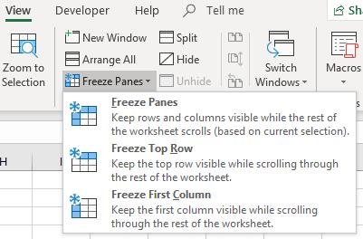
Figure 1.
Got a version of Excel that uses the ribbon interface (Excel 2007 or later)? This site is for you! If you use an earlier version of Excel, visit our ExcelTips site focusing on the menu interface.
FREE SERVICE: Get tips like this every week in ExcelTips, a free productivity newsletter. Enter your address and click "Subscribe."
Copyright © 2026 Sharon Parq Associates, Inc.
Comments