Smoothing Out Data Series

When you create line charts in Excel, the lines drawn between data points tend to be very straight. (This makes sense; the lines are meant to connect the points.) You can give your graphs a more professional look by simply smoothing out the curves Excel uses at each data point. Follow these steps if you are using Excel 2007 or Excel 2010:

1. In your chart, right-click on the data series that you want to smooth. Excel displays a Context menu.
2. Choose Format Data Series from the Context menu. Excel displays the Format Data Series dialog box.
3. Click Line Style at the left side of the dialog box. (See Figure 1.)



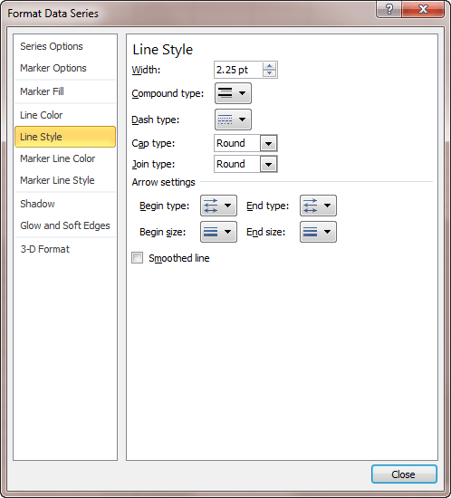
Figure 1. The Line Style options of the Format Data Series dialog box.

4. Select the Smoothed Line check box.
5. Click on OK.

The steps are slightly different in Excel 2013 and later versions:

1. In your chart, right-click on the data series that you want to smooth. Excel displays a Context menu.
2. Choose Format Data Series from the Context menu. Excel displays the Format Data Series task pane at the right side of the screen.
3. Click the Fill and Line icon (it looks like a spilling paint can).
4. Click Line to make sure the line options are visible. (See Figure 2.)



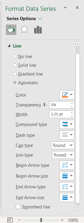
Figure 2. The Line options of the Format Data Series task pane.

5. Select the Smoothed Line check box, which is at the very bottom of the options.
6. Click on OK.

One final note: Just because Excel provides a way for you to smooth the lines connecting data points, that doesn't always mean that you should. Make sure you give some thought to what conclusions people may draw from your data. If the data in the chart is more precise with unsmoothed lines, then you should probably not smooth them. You want to avoid misrepresenting your data or causing readers to draw incorrect conclusions.

ExcelTips is your source for cost-effective Microsoft Excel training. This tip (9510) applies to Microsoft Excel 2007, 2010, 2013, 2016, 2019, and Excel in Microsoft 365. You can find a version of this tip for the older menu interface of Excel here: Smoothing Out Data Series.