Written by Allen Wyatt (last updated December 4, 2021)
This tip applies to Excel 2007, 2010, 2013, 2016, 2019, and 2021
If Jerry clicks in the Formula bar, Excel highlights the cells used in the formula, if they are on the same worksheet as the formula. Jerry wonders if there is a way to have this highlight work if the cells are on a different worksheet. He uses two monitors so he can see both worksheets at the same time.
There is no way to do this in Excel; it just isn't part of the feature that Jerry notes. There may be a workaround, however, if you work with the Formula Auditing capabilities of the program. All you need to do is select the cell containing the formula you want to analyze. When you click the Trace Precedents tool (on the Formulas tab of the ribbon), Excel displays arrows that indicate the cells contributing to the formula in the selected cell. If the arrow is dashed (not solid), then the contributing cell is in a different worksheet. (See Figure 1.)
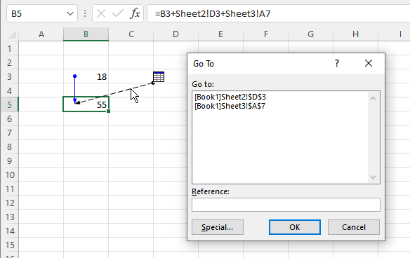
Figure 1. After double-clicking a dashed precedent line.
Double-click the dashed line, and Excel displays a Go To dialog box that contains sheet and cell references from the formula. Select one of the references, and when you click on OK (to dismiss the Go To dialog box), you are taken to that cell.
ExcelTips is your source for cost-effective Microsoft Excel training. This tip (12498) applies to Microsoft Excel 2007, 2010, 2013, 2016, 2019, and 2021.

Dive Deep into Macros! Make Excel do things you thought were impossible, discover techniques you won't find anywhere else, and create powerful automated reports. Bill Jelen and Tracy Syrstad help you instantly visualize information to make it actionable. You�ll find step-by-step instructions, real-world case studies, and 50 workbooks packed with examples and solutions. Check out Microsoft Excel 2019 VBA and Macros today!
Want to add a bunch of blank rows to your data and have those rows interspersed among your existing rows? Here's a quick ...
Discover MoreNamed ranges can make it easier to refer to ranges of cells in an understandable way. If you want to delete named ranges ...
Discover MoreNeed to concatenate the contents in a number of columns so that it appears in a single column? Excel has no intrinsic way ...
Discover MoreFREE SERVICE: Get tips like this every week in ExcelTips, a free productivity newsletter. Enter your address and click "Subscribe."
2021-12-07 06:38:05
Alex B
It might be worth adding that after the step in the quote below <F5> then <Enter> will get you back to the original cell containing your formula.
"Select one of the references, and when you click on OK (to dismiss the Go To dialog box), you are taken to that cell."
2021-12-04 13:27:00
Tomek
It should be obvious but:
Do not run any of the remove highlight macros if you didn't run the HighlightExtPrecedents first.
2021-12-04 09:20:36
Here is the promised code:
=======================
Global LastOrigin As Range
'--------------------------------
Sub HighlightExtPrecedents()
Dim rOrigin As Range
Dim LinkN As Integer
ActiveSheet.ClearArrows
Set rOrigin = ActiveCell
rOrigin.ShowPrecedents
On Error Resume Next
Do
LinkN = LinkN + 1
rOrigin.NavigateArrow TowardPrecedent:=True, ArrowNumber:=1, LinkNumber:=LinkN
If Err.Number <> 0 Then Exit Do
If rOrigin.Parent.Name = ActiveCell.Parent.Name Then
MsgBox "No precedents found on other sheets."
Exit Do
End If
CondHighlight
Loop
Set LastOrigin = rOrigin
ActiveSheet.ClearArrows
End Sub
'--------------------------------
Public Sub RemoveLastHighlight()
Dim rOrigin As Range
Dim LinkN As Integer
If LastOrigin Is Nothing Then
MsgBox "There is no record of precedent highlighting!"
Exit Sub
End If
ActiveSheet.ClearArrows
Set rOrigin = LastOrigin
rOrigin.ShowPrecedents
On Error Resume Next
Do
LinkN = LinkN + 1
rOrigin.NavigateArrow TowardPrecedent:=True, ArrowNumber:=1, LinkNumber:=LinkN
If Err.Number <> 0 Then Exit Do
If rOrigin.Parent.Name = ActiveCell.Parent.Name Then Exit Do
RemoveCondHighlight
Loop
ActiveSheet.ClearArrows
Set LastOrigin = Nothing
End Sub
'--------------------------------
Sub RemovePrecedentsHighlight()
Dim rOrigin As Range
Dim LinkN As Integer
ActiveSheet.ClearArrows
Set rOrigin = ActiveCell
rOrigin.ShowPrecedents
On Error Resume Next
Do
LinkN = LinkN + 1
rOrigin.NavigateArrow TowardPrecedent:=True, ArrowNumber:=1, LinkNumber:=LinkN
If Err.Number <> 0 Then Exit Do
If rOrigin.Parent.Name = ActiveCell.Parent.Name Then Exit Do
RemoveCondHighlight
Loop
Set LastOrigin = rOrigin
ActiveSheet.ClearArrows
End Sub
'--------------------------------
Public Sub CondHighlight()
Selection.FormatConditions.Add Type:=xlExpression, Formula1:="=TRUE"
Selection.FormatConditions(Selection.FormatConditions.Count).SetFirstPriority
With Selection.FormatConditions(1).Interior
.Color = RGB(255, 200, 255)
End With
Selection.FormatConditions(1).StopIfTrue = True
End Sub
'--------------------------------
Public Sub RemoveCondHighlight()
Selection.FormatConditions(1).Delete
End Sub
2021-12-04 09:19:26
Tomek
The answer provided in Allens tip did not quite provide a solution for Jerry to be able to see all precedent cells on other sheets highlighted and visible in additional Excel windows. I have a macro solution for that. It is a bit extensive but hopefully would be useful for Jerry.
I am proposing to use the conditional formatting to highlight the precedent cells. Regular background and borders could be used, but any conditional formatting already applied to the precedent cells would take precedence over any explicit formatting. Also, the conditional formatting must be applied in such a way that it will take precedence over any existing conditional formatting. As a bonus, when this particular highlighting rule for conditional formatting is removed, the original formatting, whether explicit or conditional is simply restored, without any need to store then recall the cell formatting that existed before highlighting.
The solution consists of several macros. Here is how it works:
The macro HighlightExtPrecedents will first show precedent arrows for the selected cell; if a range of cells was selected only the active cell will be used. I will call this cell “origin cell” in the rest of this description. The macro will follow the arrow to the precedent ranges or cells on other sheets. In my testing I found that all precedents from other sheets are pointed to by ArrowNumber 1. The remaining arrows point to precedents on the same sheet. This was tested in MS365 Family under Win10; older versions of Excel may behave differently regarding arrow numbers, but I have no access to them to test. Also, if there is no precedent from another sheet, the ArrowNumber 1 points to the first precedent on the same sheet; the macro tests for this and does not do any highlighting in such case, just displays a message: “No precedents found on other sheets.”
The second macro (RemoveLastHighlight) removes the highlighting that was ***last*** applied. This makes it easy to remove last highlighting without having to navigate to the origin cell. The location of the origin cell is stored in a Global variable LastOrigin by the HighlightExtPrecedents procedure and is used and reset to Nothing by the RemoveLastHighlight procedure. The content of the global variable may be lost in some situations (e.g., when the Reset button in VBA editor window is pressed or after a run-time error) and is also lost if the workbook is closed. The macro will notify the user of the fact there is no record about last highlighting. In such case the user should run a slightly different un-highlighting macro, as described next.
The macro RemovePrecedentHighlight unhighlights the precedents from other sheets using the same logic as highlighting. Before running the macro, the user ***must*** select the same cell that was selected as origin for highlighting, as it will remove border and background formatting for precedents of currently selected cell.
Highlighting and removing highlight is meant to work in tandem to provide a temporary indication where the precedent cells are. If changes to formulas are made in between the two actions, or if the macros are not run in proper sequence, they may each act on wrong precedent cells and result in fouling up the highlighting.
The two additional subs: CondHighlight and RemoveCondHighlight, are called to apply or remove, respectively, conditional formatting to/from a cell or range selected by the loop in one of the main subroutines. Separation of CondHighlight from the main sub makes it easier for the user to modify the highlighting color and/or adding additional highlighting attributes like border.
One additional comment on using this solution with multiple monitors, or more precisely, multiple Excel windows: It works best if the origin cell is selected in Window #1. If it is in any other window, that window may return view to the origin sheet. Not really a big deal, but it is nicer if the highlighted cells stay visible on other sheets.
I am going to post the code as my separate comment to be able to format it better.
Got a version of Excel that uses the ribbon interface (Excel 2007 or later)? This site is for you! If you use an earlier version of Excel, visit our ExcelTips site focusing on the menu interface.
FREE SERVICE: Get tips like this every week in ExcelTips, a free productivity newsletter. Enter your address and click "Subscribe."
Copyright © 2025 Sharon Parq Associates, Inc.
Comments