Please Note: This article is written for users of the following Microsoft Excel versions: 2007, 2010, 2013, 2016, 2019, 2021, 2024, and Excel in Microsoft 365. If you are using an earlier version (Excel 2003 or earlier), this tip may not work for you. For a version of this tip written specifically for earlier versions of Excel, click here: Changing the Color of Worksheet Gridlines.
Written by Allen Wyatt (last updated May 10, 2025)
This tip applies to Excel 2007, 2010, 2013, 2016, 2019, 2021, 2024, and Excel in Microsoft 365
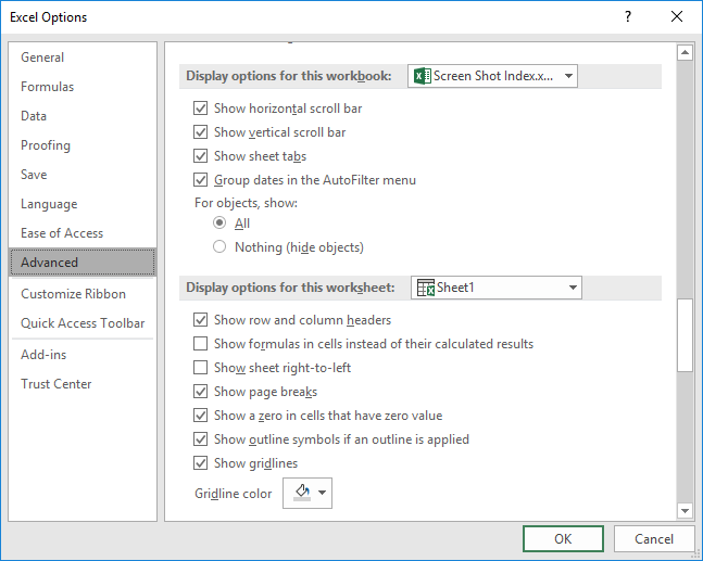
Most people using Excel leave the gridlines visible so that they can easily see where the various cells are. By default, the gridlines are a light gray. You can easily change the gridlines to a different color by following these steps:

Figure 1. The Advanced options of the Excel Options dialog box.
ExcelTips is your source for cost-effective Microsoft Excel training. This tip (6210) applies to Microsoft Excel 2007, 2010, 2013, 2016, 2019, 2021, 2024, and Excel in Microsoft 365. You can find a version of this tip for the older menu interface of Excel here: Changing the Color of Worksheet Gridlines.

Excel Smarts for Beginners! Featuring the friendly and trusted For Dummies style, this popular guide shows beginners how to get up and running with Excel while also helping more experienced users get comfortable with the newest features. Check out Excel 2019 For Dummies today!
Want a quick way to combine your worksheets? This tip features a simple macro to do the task for you.
Discover MoreEver want to use the name of a worksheet tab within a cell? Here's how you can access that information using the CELL ...
Discover MoreWant to make fast work of moving from one worksheet to another? Here's how to do the task when you have a lot of ...
Discover MoreFREE SERVICE: Get tips like this every week in ExcelTips, a free productivity newsletter. Enter your address and click "Subscribe."
2025-06-05 19:23:35
Kevin H
On Mac, this is under Excel > Preferences > View
2025-05-12 05:02:35
DaveS
@Ray
Two ways of doing that are:
(i) Under the Borders dropdown (Home tab of the ribbon), select Draw Border Grid, then select the range of cells you want and it infills the borders. Default is black but if you select Line color first to set another colour.
(ii) Select the range of cells and then under the Format dropdown (Home tab of the ribbon) select Format Cells to open the Format Cells dialog, and then select the Border tab on the dialog. This approach enables whole rows or columns to be selected whereas I think (i) only works on blocks of cells.
2025-05-10 06:36:20
Ray McAllister
Can I change the color of grid lines in different parts. Of a worksheet? That is, can I make grid lines red for some rows (or columns) and blue for others?
Got a version of Excel that uses the ribbon interface (Excel 2007 or later)? This site is for you! If you use an earlier version of Excel, visit our ExcelTips site focusing on the menu interface.
FREE SERVICE: Get tips like this every week in ExcelTips, a free productivity newsletter. Enter your address and click "Subscribe."
Copyright © 2026 Sharon Parq Associates, Inc.
Comments