Listing the Top Five Transactions

Terri has a list of transactions in a worksheet. The first column is a customer name and the second is the transaction amount. Terri knows she could sort or filter the data to determine the top five transactions. However, she wonders if the top five customers and the transaction amount could actually be returned by a formula.

Yes, it is possible to do this and there are many different ways you can approach the problem. In this tip I'm going to look at only a few of those approaches.

First, though, let's make the assumption that the customer names are in column A and that cell A1 has a header in it, such as "Customer." Further, column B contains a header of "Amount" and the rest of the column contains the amounts for each corresponding customer in column A. (See Figure 1.)

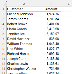
Figure 1. Sample data for testing formulas.

Now, let's take a look at an approach that will work in all versions of Excel. Start by placing the values 1, 2, 3, 4, 5 in cells D2:D6. These are your "rank" indicators. Then, in cell F2 you can place the following formula:

=LARGE(B:B,D2)

Copy this formula down to cell F6, and you end up with the five largest transactions in F2:F6. This is because the LARGE function returns the Nth largest value from a range, where the second parameter indicates the rank—in this case 1, 2, 3, 4, or 5.

Now all you need to do is to grab the names related to those transaction amounts. You can do that by putting this formula into cell E2:

=INDEX(A:A,MATCH(F2,B:B,0))

Copy this down to cell E6. The MATCH function matches the amounts in column F against the amounts in column B, and then the INDEX function pulls the corresponding name from column A. You end up with the desired names and transaction amounts in E2:F6. You can even put headers in cells D1:F1, if desired, and format as necessary. (See Figure 2.)

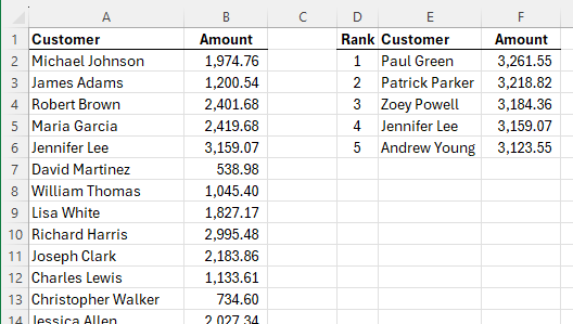
Figure 2. Pulling the top five transactions.

If you are using Excel 2021, 2024, or Excel in Microsoft 365, then you can rely on the newer worksheet functions that are available. A single formula can be used to return the desired information. Here's the one I would place in cell E2:

=FILTER(A2:B1000, B2:B1000 >= LARGE(B2:B1000,5))

The key here is to make sure that the ranges specified include all of the rows in your data. In this case, the range evaluated is A2:B1000, but you can adjust this as needed. The formula returns the top five transactions, though it may return more if there are duplicate transaction amounts in the top five. They are returned in the same order that they appear in the original data. If you would, instead, like them sorted in descending order by the transaction amount, you can wrap the formula in the SORT function:

=SORT(FILTER(A2:B1000,B2:B1000>=LARGE(B2:B1000,5)),2,-1)

Here's another approach that will work in Excel 2021, 2024, and Excel in Microsoft 365, relying on both the SORT and SEQUENCE functions:

=INDEX(SORT(A2:B1000,2,-1), SEQUENCE(5),{1,2})

If you are using Excel in Microsoft 365, then you will have access to the TAKE function, which can shorten the formula even more:

=TAKE(SORT(A2:B1000,2,-1),5,2)

This formula provides a sorted array of the cells, in descending order based on the transaction amount, and then "takes" the first five rows and two columns.

ExcelTips is your source for cost-effective Microsoft Excel training. This tip (9261) applies to Microsoft Excel 2007, 2010, 2013, 2016, 2019, 2021, 2024, and Excel in Microsoft 365.