Please Note: This article is written for users of the following Microsoft Excel versions: 2007, 2010, 2013, 2016, 2019, 2021, and Excel in Microsoft 365. If you are using an earlier version (Excel 2003 or earlier), this tip may not work for you. For a version of this tip written specifically for earlier versions of Excel, click here: Conditional Formatting Based on Date Proximity.
Written by Allen Wyatt (last updated October 5, 2023)
This tip applies to Excel 2007, 2010, 2013, 2016, 2019, 2021, and Excel in Microsoft 365
Richard wondered if it was possible, using conditional formatting, to change the color of a cell. For his purposes he wanted a cell to be red if it contains today's date, to be yellow if it contains a date within a week of today, and to be green if it contains a date within two weeks.
You can achieve this type of conditional formatting if you apply a formula. For instance, let's assume that you want to apply the conditional formatting to cell A1. Just follow these steps:
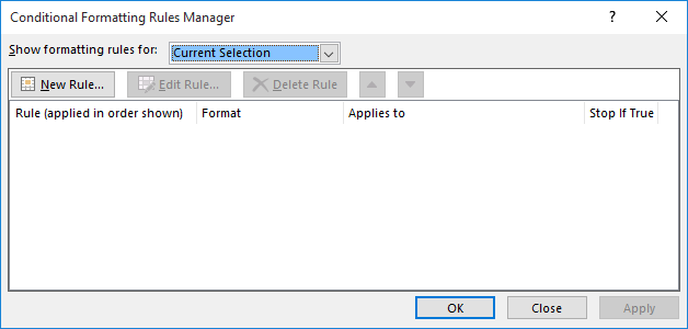
Figure 1. The Conditional Formatting Rules Manager dialog box.
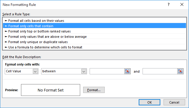
Figure 2. The New Formatting Rule dialog box.
One important thing to bear in mind with conditional formatting is that criteria are evaluated in the order in which they appear. Once a criterion has been met, then the formatting is applied and other criteria are not tested. It is therefore important to set out the tests in the correct order. If, in the example above, the criteria had been entered in the reverse order, i.e. test for 14 days, then 7 and then 0, it would have only applied the 14 days format even if the date entered was today. In other words, if the date is today then all three of the tests would have been met so you have to be careful of the order in order to get the result you need.
ExcelTips is your source for cost-effective Microsoft Excel training. This tip (6287) applies to Microsoft Excel 2007, 2010, 2013, 2016, 2019, 2021, and Excel in Microsoft 365. You can find a version of this tip for the older menu interface of Excel here: Conditional Formatting Based on Date Proximity.

Dive Deep into Macros! Make Excel do things you thought were impossible, discover techniques you won't find anywhere else, and create powerful automated reports. Bill Jelen and Tracy Syrstad help you instantly visualize information to make it actionable. You�ll find step-by-step instructions, real-world case studies, and 50 workbooks packed with examples and solutions. Check out Microsoft Excel 2019 VBA and Macros today!
When preparing a report for others to use, it is not unusual to add a horizontal line between major sections of the ...
Discover MoreConditional Formatting is a great boon to effectively displaying the information in your worksheets. If you want to ...
Discover MoreThere are many times when you are creating a worksheet that you need to analyze dates within that worksheet. Once such ...
Discover MoreFREE SERVICE: Get tips like this every week in ExcelTips, a free productivity newsletter. Enter your address and click "Subscribe."
2020-10-26 16:54:16
Ali
Thank you, super helpful! The summary worked well. There was one part that was unclear (not sure if it is because I have a Mac version of the Office Suite), I had to click on "Classic" in order to find the formatting type.
Is there a way to automate a report from this? Say that the I want a report to run daily to summarize and rows that have a red cell? I assume there is a way, so a better question is whether someone without experience writing scripts can pull this off?
2020-10-26 12:10:51
Ali
Thank you, super helpful! The summary worked well. There was one part that was unclear (not sure if it is because I have a Mac version of the Office Suite), I had to click on "Classic" in order to find the formatting type.
Is there a way to automate a report from this? Say that the I want a report to run daily to summarize and rows that have a red cell? I assume there is a way, so a better question is whether someone without experience writing scripts can pull this off?
2020-10-26 10:51:25
Ali
Thank you, super helpful! The summary worked well. There was one part that was unclear (not sure if it is because I have a Mac version of the Office Suite), I had to click on "Classic" in order to find the formatting type.
Is there a way to automate a report from this? Say that the I want a report to run daily to summarize and rows that have a red cell? I assume there is a way, so a better question is whether someone without experience writing scripts can pull this off?
2020-10-22 12:32:49
Toba
Thanks for the tips. Very valuable for me. Just use for a quick working excel file.
2020-01-04 15:54:08
J. Woolley
@Robert Nye (part 2)
Assuming the cells containing your dates are $D$1:$D$25, the final conditional formatting rules should look like this:
(see Figure 1 below)
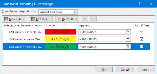
Figure 1.
2020-01-04 15:49:13
J. Woolley
@Robert Nye
Select the cells containing your dates, then apply these 3 rules using procedures described in the Tip:
(see Figure 1 below)
(see Figure 2 below)
(see Figure 3 below)
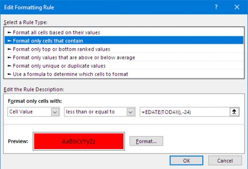
Figure 1.
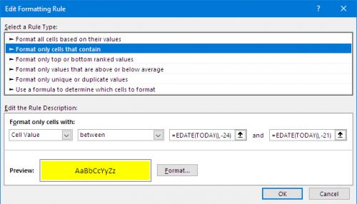
Figure 2.
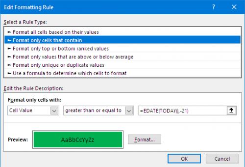
Figure 3.
2020-01-03 14:49:42
Robert Nye
I am trying to get a cell to change colors depending on the date. I will put a certification date in a cell, i need that cell to be green from the date entered to 21 months past the date entered than i need the date to be yellow from 21 months past to 24 months past and red for anything past 24 months. could i get help with this formula please.
Thank you.
2019-05-01 07:53:58
Alan Bahnam
Ok, I am stumped, I have used this formula and I cannot get it to work properly. I have a column (m33 Order Survey) which will get a date when the survey gets ordered, then I have a column (o33 Rcv Survey). I need the m33 column to turn green when the initial date is entered and turn red after 12 days if the (o33 Rcv Survey) never gets a date or date entered exceeds 12 days. Please help. Thanks
2019-01-03 08:53:52
Peter Atherton
Natalie
I forget to say that You base the condiional format on the helper column
2019-01-03 08:48:31
Peter Atherton
Natalie
Assuming that the dates are in column B and the entry date is in column C, try this
Private Sub Worksheet_Change(ByVal Target As Range)
Dim dt As Date
dt = Now
dt = Format(dt, "dd/mm/yyyy")
If Target.Column <> 2 Then Exit Sub
Target.Offset(0, 1).Value = dt
End Sub
Right-click the worksheet Tab and select the View Code and paste the code into the module.
HTH
2019-01-01 17:37:34
Natalie
I need to know how to format cells (change cell color) based on DATE OF ENTRY.
Like, say the date I have entered is 1/15/19 but the date I ENTERED the text is 1/3/19... that is what I need to format.
I need to format the cells so that they change color after 30 days have passed since ORIGINAL ENTRY DATE, as opposed to the actual date entered.
Does that make sense? Is there even a way to do it?
It's driving me crazy. I appreciate the help!
2018-04-13 07:03:53
Bobby O,
Depending on how stringent your requirements for conditional formatting are, the following will work. Assuming the cell containing your start date is named as startdate.
=AND(ISNUMBER(D4),D4<>startdate)
As excel stores dates as a number (regardless of what is displayed on screen) any number will trigger the conditional formatting. If you want to limit the permitted dates you can add another AND condition such as "<=startdate+365" (without the quotes) would only trigger formatting if the date is within a year of the startdate.
HTH
Steve
2018-04-12 16:12:43
Bobby O
it was possible, using conditional formatting, to change the color of a cell when you type any date in the cell.
for instance, I have Cells A2:G34 highlighted in Light Gray. When I type a date (any date) other than the Start Date,
I want the color to turn Green.
What formula would you suggest?
Thank you,
BobbyO
2018-03-02 05:21:13
Steve Jez
Jake,
Three rules,
Select F2:F35
Conditional Formatting
Use formula to determine which cells to format
New Rule
=F5>TODAY()+60 (Format fill Green)
=AND(F5>=TODAY()+31,F5<=TODAY()+60) (Format fill Yellow)
=F5<=TODAY()+30 (Format fill Red)
Hope this helps
Steve
2018-03-01 10:03:59
Jake
I am military and we have certs that last a year and some items that have expiration dates.
I have these in separate columns so that I can format them to turn red when the expiration date is within 30 days, turns yellow 31-60 days from expiration and, green for anything greater than 61+ days. I have followed the formulas and even skipped steps 5 and 6 as suggested for bill. they are in Colum F and go from row 2 to row 35.
I can not get them to turn any colors at all. what would my manage rules tab look like.
2017-05-10 03:02:20
Steve J
Colin.
The formula you need is
=AND(A5="",A4<=TODAY()-30)
Adjust cell references as required.
It checks that A5 is blank AND A4 is older or equal to today.
HTH
Steve
2017-05-09 22:09:31
Colin
I want to change a cell red when the date has passed 30 days on the condition that another cell date has not been entered yet. I have looked online a lot and can't find out how to do it.
2017-01-07 06:37:26
@Bill
Your Conditional formatting rules will need to be 3 between & ignore steps 6 & 7 above. the rules should be like
cellvalue between =$D$16-30 =$D$16+30
etc etc.
The $ signs in the D16 address are essential otherwise as the formatting goes down your column of dates D16 becomes D17, D18 etc.
Also try making the first rule 30 then 60 then 90.
2017-01-05 19:58:09
Bill Nees
Mr. Wyatt
In cell D16 I have a date, 03/17/17.
This date is an expiration date.
I have tried to condition format this cell to change to green when todays date is within 90 days, and yellow within 60 days, then red within 30 days.
No matter how I arrange them, the cell stays whatever color when it gets to the first format.
Is there a way to write this formula so that it only is green from 90 to 60 days, then turns yellow from 60 to 30 days, then turns red from 30 days?
D16 never changes till I set a new expiration date.
I am a truck driver, and don’t understand much about formulas in spread sheets, although I am trying.
Thank you for your help if you can.
Thanks anyway if you can’t.
Bill
2016-06-07 18:17:10
The Original Buzz
Thank you for making my life so much easier. I use Excel more than any other program and will definitely be a regular visitor to this site.
2016-03-22 00:09:02
Sunae Hwang
Hi,
I followed the exactly but it only shows green whether enter the cell value for today's date, +-week, or +-two weeks. Why it's not working for me? I went through twice to make sure I didn't leave anything out. I am using Office 2010.
Thank you.
2016-03-20 07:22:33
I do this a lot at work in my big spread-sheet to remind me when the instruments in my care are due for calibration.
I don't set a condition for the green boxes. I just set them manually to green fill, then when the date nears, this changes to yellow, and of course(if I have overlooked one!) to RED.
And I have lots of macros on buttons to sort the instrument list by name, by asset number, by date due, etc.
Excel helps me a lot - I can't imagine life without it.
Got a version of Excel that uses the ribbon interface (Excel 2007 or later)? This site is for you! If you use an earlier version of Excel, visit our ExcelTips site focusing on the menu interface.
FREE SERVICE: Get tips like this every week in ExcelTips, a free productivity newsletter. Enter your address and click "Subscribe."
Copyright © 2025 Sharon Parq Associates, Inc.
 Please Note:
This article is written for users of the following Microsoft Excel versions: 2007, 2010, 2013, 2016, 2019, 2021, and Excel in Microsoft 365. If you are using an earlier version (Excel 2003 or earlier), this tip may not work for you. For a version of this tip written specifically for earlier versions of Excel, click here:
Please Note:
This article is written for users of the following Microsoft Excel versions: 2007, 2010, 2013, 2016, 2019, 2021, and Excel in Microsoft 365. If you are using an earlier version (Excel 2003 or earlier), this tip may not work for you. For a version of this tip written specifically for earlier versions of Excel, click here:
Comments