Automatic Lines for Dividing Lists

Let's say you have a list of company transactions. Each transaction includes a department number, a title, and other information (amount, date, authorizer, etc.). As you get more and more of these items in your list, you may want a way to automatically add "dividing lines" based on the department number. For instance, when the department number changes, you may want to include a line between the two departments.

To add this type of formatting to your list, start by sorting your data table by department. For the sake of this example, I'll assume that your data is actually in columns A:F, with the department numbers in column A. (See Figure 1.)

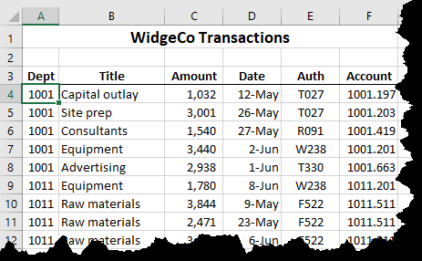
Figure 1. The data to be divided.

To add the automatic dividing lines, follow these steps:

1. Select the left-most cell of the first row of your data. For instance, if your table heads are in row 3 and your first row of data is in row 4, you should select cell A4.
2. Press Shift+Ctrl+End. All the cells in your data table should be selected, with the exception of the header row.
3. With the Home tab of the ribbon displayed, click the Conditional Formatting option in the Styles group. Excel displays a palette of options related to conditional formatting.
4. Click New Rule. Excel displays the New Formatting Rule dialog box.
5. In the Select a Rule Type area at the top of the dialog box, choose Use a Formula to Determine Which Cells to Format. (See Figure 2.)



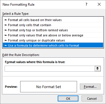
Figure 2. The New Formatting Rule dialog box.

6. In the Format Values Where This Formula Is True box, enter "=$A4<>$A5" (without the quote marks). This formula, of course, will vary depending on your data. As entered here, it is appropriate for the data table already described in this tip and the cell selected in step 1.
7. Click Format to display the Format Cells dialog box.
8. Display the Border tab.
9. Click the None button to remove any borders already applied to the cells.
10. In the Style list, select the type of border you want to appear between departments.
11. In the Border area of the dialog box, click the button that adds your selected border style to the bottom of the cells.
12. Click OK to dismiss the Format Cells dialog box. The formatting you specified in steps 10 and 11 should now appear in the preview area for the rule.
13. Click OK.

That's it; you should now see a line that appears across the entire width of your data every time the department changes.

ExcelTips is your source for cost-effective Microsoft Excel training. This tip (6863) applies to Microsoft Excel 2007, 2010, 2013, 2016, 2019, Excel in Microsoft 365, and 2021. You can find a version of this tip for the older menu interface of Excel here: Automatic Lines for Dividing Lists.