Please Note: This article is written for users of the following Microsoft Excel versions: 2007, 2010, 2013, 2016, 2019, and 2021. If you are using an earlier version (Excel 2003 or earlier), this tip may not work for you. For a version of this tip written specifically for earlier versions of Excel, click here: Easily Entering Dispersed Data.
Written by Allen Wyatt (last updated October 31, 2020)
This tip applies to Excel 2007, 2010, 2013, 2016, 2019, and 2021
I needed to enter information into many rows of widely dispersed columns, like A, Q, BD, BJ, CF, etc. (I'm sure you get the idea.) I was right-arrowing along and I was thinking: if I were in Word, I'd just set some tabs or bookmarks to move around quickly. What is the equivalent in Excel? A little delving into the Help files let me know that it's done like this:
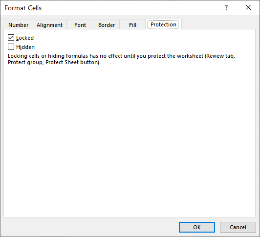
Figure 1. The Protection tab of the Format Cells dialog box.
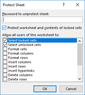
Figure 2. The Protect Sheet dialog box.
That's it! Excel will only let you go to cells that are still editable, and those are the ones for which you cleared the Lock property before you protected the sheet. Enjoy tabbing to the places on your worksheet that you need to.
ExcelTips is your source for cost-effective Microsoft Excel training. This tip (9364) applies to Microsoft Excel 2007, 2010, 2013, 2016, 2019, and 2021. You can find a version of this tip for the older menu interface of Excel here: Easily Entering Dispersed Data.
Program Successfully in Excel! John Walkenbach's name is synonymous with excellence in deciphering complex technical topics. With this comprehensive guide, "Mr. Spreadsheet" shows how to maximize your Excel experience using professional spreadsheet application development tips from his own personal bookshelf. Check out Excel 2013 Power Programming with VBA today!
Delete a cell or a range of cells, and Excel needs to figure out how to rearrange the void left by the deletion. You can ...
Discover MoreHave a worksheet in which there may be entire columns that are duplicates of each other? If you want to delete those ...
Discover MoreExcel makes it easy to copy and paste a range of cells. Easy, that is, unless the range isn't contiguous. If you have a ...
Discover MoreFREE SERVICE: Get tips like this every week in ExcelTips, a free productivity newsletter. Enter your address and click "Subscribe."
2021-02-13 12:13:37
Roy
For the described problem, one pictures entering a set of data. The simple version would be all in the same row, but to make life hard, varying data sets might leave related items in different rows.
Any time I need anything that seems to fit that bill, I set up a Named Range for one set of the cells. I select a cell IN the set of cells so all the references proerply relate to each other and I use relative references to all cells. Then when I need to do the entries, I use the Named Range box to the left of the editing bar to select the Named Range.
Say I set it up using cells A1, D4, and J23. I set up the range, first selecting the uppermost left cell of them (so my references will never roll up or left past the upper and left edges of the usual layout, and create the Named Range. More in a moment. If I then select the range from the box, the cells in the range are selected and I can enter my set of data using TAB or Enter to move between cells in the range.
Points of interest:
1. First and foremost, like many other Windows things, if you present Windows a list (and Excel in this case), it will act upon the LAST item first, then do the list in the order one would expect. So to have A1 (for this example) highlighted when the range is selected, it has to be the last listed cell in the range. So, for example: D4, J23, A1 highlights with A1 the selected cell.
2. Except for that, if one likes, one can order the cells in the range in the order one wishes to traverse them. Perhaps I wish to start in A1 and move to J23 (as in, NOT D4 next), then to D4. So I'd enter the range as: J23, D4, A1.
3. One can even go to a cell more than once in the TAB/Enter cycling by entering it extra times in appropriate order (though the highlighting looks different that usual.
4. Because relative addressing was used, relative sets are selected, not absolute ones. So select (click in) cell A3, then select the range, and cells A3, J25, D6 are selected. This is a hugely nice thing when it comes to entering SETS of data.
5. If one ever found a use for it, you CAN mix relative and absolute addressing, so J23, $D$4, A1 selects A1, D4, J23 if A1 ia selected before selecting the range, and then for A3 having been selected when selecting the range, A3, D4, J25 are selected.
I don't actually use it for data entry much anymore since almost everything I use is MY writing nowadays, but back when slaved to other people's concepts for laying out spreadsheets, it was a Godsend. However, I DO have uses in which I enter data in an area of a spreadsheet which I then need to clear for the next batch of work. Usually such a thing has odd "not-in-a-rectangle" bits. By declaring a Named Range, I can simply select it which highlights everything I could have entered something in, then pressing Delete clears anything I might've entered so absolutely nothing can be mistakenly left behind to mess up the next bit of work
(Remember that NFL commercial from something like five years ago? A set of football players wearing vaguely college-y uniforms is hammering away in practice and the voiceover says "They practice until the get it right." Then a set of football palyers wearing more vibrant uniforms, more "pro" ia shown, hammering away in practice (but clearly much more elite in speed and power, even the things they are doing) and the voiceover says "We practice until we can't get it wrong." That summed it up in a nutshell. Why should I EVER have to tell the boss "Sorry man, I left a cell behind after I did the first analysis and it ruined the second analysis, just not garishly enough to be clearly wrong."?)
It is also useful for EDITING a set of data that doesn't appear in obviously related geometry as it highlights the full data set, allows moving between only those cells, and there is no editing just a row above or below by accident. Even if everything is in a single row, this is handy, if only in that "we can't get it wrong" sense. And very handy if there are clumped entries that are very similar, but your editing is only interested in one of them (for instance, there're columns next to each other for ship by date, promise date, due date, etc. and you could see someone changing the wrong one 'cause"Iit was a date, man, I didn't notice it wasn't the right date, man."
But make SURE you click into that upper left cell before setting the Named Range if using the relative addressing. Otherwise you will get fuuny things. And sometimes you will anyway, so you have to set the Named Range even 2-3 times before it finally works. Then first time, every time for six months before Excel just acts funny again. I honestly think that's due to how long you've had the program running, how long you've used it without restarting, but have no real evidence for it. It WILL always take after a couple, three tries, but I've taken to saving, closing Excel, and restarting whereupon it always takes immediately. I figure if that feature was going south, others might've been doing so as well, so it's worth it. Instability... what would it be like to use an MS product without instability. I'm sure I'll never know...
By the way, that all sounds obnoxious, probably due to how long it is and the list of notes, but it takes just 30 seconds for a simple range.
2020-11-15 10:15:56
JMJ
Yes, I agree with JC: I certainly would have hidden the useless columns...
2020-11-02 10:44:10
JC
How about temporarily hiding columns that don't need data entry?
2020-10-31 19:06:10
Peter
A good and likely useful trick.
Depending on the nature of the model, you could just have a data entry tab and refer to the data entry cells by formula. This gives you the opportunity to modify the values as well, say, from imperial to metric or perhaps apply data validation.
Got a version of Excel that uses the ribbon interface (Excel 2007 or later)? This site is for you! If you use an earlier version of Excel, visit our ExcelTips site focusing on the menu interface.
FREE SERVICE: Get tips like this every week in ExcelTips, a free productivity newsletter. Enter your address and click "Subscribe."
Copyright © 2025 Sharon Parq Associates, Inc.
 Please Note:
This article is written for users of the following Microsoft Excel versions: 2007, 2010, 2013, 2016, 2019, and 2021. If you are using an earlier version (Excel 2003 or earlier), this tip may not work for you. For a version of this tip written specifically for earlier versions of Excel, click here:
Please Note:
This article is written for users of the following Microsoft Excel versions: 2007, 2010, 2013, 2016, 2019, and 2021. If you are using an earlier version (Excel 2003 or earlier), this tip may not work for you. For a version of this tip written specifically for earlier versions of Excel, click here:
Comments