Written by Allen Wyatt (last updated February 3, 2026)
This tip applies to Excel 2007, 2010, 2013, 2016, 2019, 2021, and Excel in Microsoft 365
Roland is looking for a way to create a list of every other Tuesday through an entire year. Fortunately, there are many ways you can come up with every other Tuesday. The first is to simply use a formula to do the dates for you, as is done in these steps:
That's it; the dates are all Tuesdays—every other Tuesday—because you've added 14 (the number of days in two weeks) to the previous Tuesday's date. This approach has a benefit, as well: If you change the date in cell A2, then all the other dates change, as well. This allows you to have a dynamic set of dates, each date two weeks later than the previous date.
If you don't need the list to be dynamic, then you can create a list of dates in this manner:
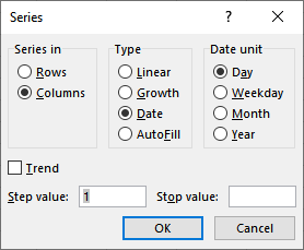
Figure 1. The Series dialog box.
The result is that Excel fills all the selected cells with dates that are 14 days apart from each other. Another way to display the same Series dialog box is to perform step 1 and then right-click on the Fill handle and drag it downward. When you release the mouse button, a Context menu appears. Choose Series, and the Series dialog box appears. You can then continue with steps 4 and 5.
If you'd rather not mess with the Series dialog box, there is a shortcut way of accomplishing the same task using the Fill handle:
When you release the Fill handle, Excel fills those cells with dates that are patterned after the two dates in cells A2:A3. Since those dates are two weeks apart, the filled dates will also be two weeks apart.
ExcelTips is your source for cost-effective Microsoft Excel training. This tip (11783) applies to Microsoft Excel 2007, 2010, 2013, 2016, 2019, 2021, and Excel in Microsoft 365.

Solve Real Business Problems Master business modeling and analysis techniques with Excel and transform data into bottom-line results. This hands-on, scenario-focused guide shows you how to use the latest Excel tools to integrate data from multiple tables. Check out Microsoft Excel Data Analysis and Business Modeling today!
Want to convert an elapsed time, such as 8:37, to a decimal time, such as 8.62? If you know how Excel stores times ...
Discover MoreIf you store dates in your worksheets, you may want to update those dates at the end of the year. This tip explains ...
Discover MoreBecause Excel stores dates internally as serial numbers, it makes doing math with those dates rather easy. Even so, it ...
Discover MoreFREE SERVICE: Get tips like this every week in ExcelTips, a free productivity newsletter. Enter your address and click "Subscribe."
There are currently no comments for this tip. (Be the first to leave your comment—just use the simple form above!)
Got a version of Excel that uses the ribbon interface (Excel 2007 or later)? This site is for you! If you use an earlier version of Excel, visit our ExcelTips site focusing on the menu interface.
FREE SERVICE: Get tips like this every week in ExcelTips, a free productivity newsletter. Enter your address and click "Subscribe."
Copyright © 2026 Sharon Parq Associates, Inc.
Comments