Written by Allen Wyatt (last updated March 5, 2024)
This tip applies to Excel 2007, 2010, 2013, 2016, 2019, 2021, and Excel in Microsoft 365
David wonders what the difference is between tables and named ranges and why he would prefer one over the other. He currently uses ranges are named, of course, and they are dynamic when it suits his purposes (most of the time).
There is probably quite a bit about tables that could be written—probably much more than what I'll choose to write here. The bottom line is that a named range can be very powerful in formulas. However, a table encompasses named ranges (they are utilized in how Excel defines tables) and adds quite a bit more functionality.
To understand what I mean, let's take a look at how you create a table. It is not uncommon to have data in Excel that is quite "tabular." It consists of rows and columns, with the first row used to add column headings. (See Figure 1.)
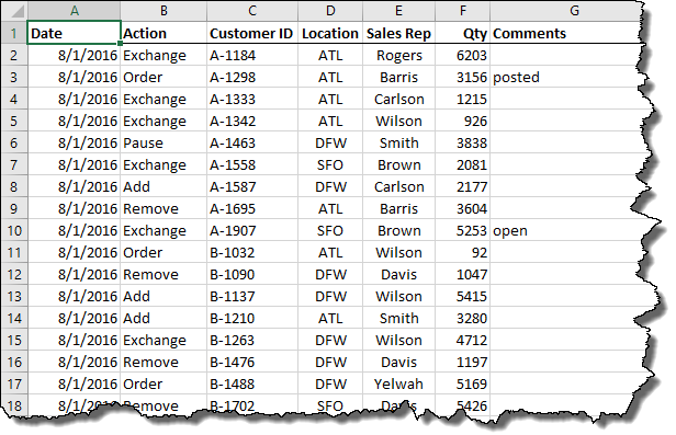
Figure 1. Sample data in a worksheet.
You convert this data to a table by selecting any cell in the data and then clicking the Table tool on the Insert tab of the ribbon. Excel asks you to confirm that you want to convert the data to a table, and when you click on OK the deed is done. (See Figure 2.)
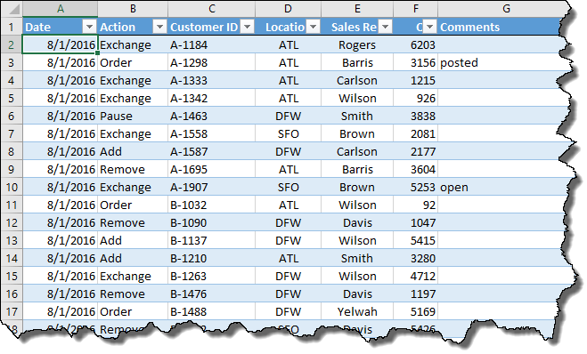
Figure 2. Sample data in a defined table.
You can tell it is now a table because Excel formats the data differently than it was before. It is now "banded" using alternating rows of color, designed to make it easier to keep your place as you work with the data.
Note, as well, that there are filter arrows at the right side of each column. This is something you cannot do with named ranges: filter the data as an inherent part of the range. If you click a down-arrow next to a column, you'll see different ways to sort and filter the data in the table based on the contents of that column.
You'll also notice that the ribbon has changed; there is now a Design tab, which should be selected. At the left side of the ribbon, in the Properties group, you see the name which Excel has assigned to your new table. It defaults to something like "Table1" or "Table2," but you should change the name to something more descriptive of the data in your table. This is, essentially, a named range that applies to the table as a whole.
As you start to work with the table, you'll notice other differences, as well. Here's a few of them:
Another neat feature is that you can use "shorthand" in your table formulas. So, instead of specifying cell references in a formula, you could do something like this:
=[@Qty]*1.25
The brackets indicate you are using the shorthand code, which consists of the @ sign followed by the name of the column defined in your header. This can make for much easier-to-read formulas in the table.
This should give you a quick idea of how defined tables differ in usage from named ranges. Like I said, there is much more that could be written about the differences, but the best way to find out is to start using tables for your data and see how they fit into your actual use of Excel.
There is one "gotcha" you need to be aware of, however. If you use tables in a workbook, you cannot share that workbook with others. Excel requires tables to be converted to named ranges if you decide to share the workbook with others.
ExcelTips is your source for cost-effective Microsoft Excel training. This tip (13476) applies to Microsoft Excel 2007, 2010, 2013, 2016, 2019, 2021, and Excel in Microsoft 365.

Excel Smarts for Beginners! Featuring the friendly and trusted For Dummies style, this popular guide shows beginners how to get up and running with Excel while also helping more experienced users get comfortable with the newest features. Check out Excel 2019 For Dummies today!
Sometimes it is necessary to print a worksheet to see how the data it contains appears. This may not be necessary, ...
Discover MoreNeed to test your formulas? Then you need some testing data that you can use to see if the formulas function as you ...
Discover MoreNeed to clear out a large amount of information saved on the Clipboard? All you need to do is to replace it with a small ...
Discover MoreFREE SERVICE: Get tips like this every week in ExcelTips, a free productivity newsletter. Enter your address and click "Subscribe."
2024-03-05 05:26:43
Barry
Once again I thank Allen and all who participate in this and other .Tips. On most occasions I find something new to me.
On a different issue but demonstrated in this Tip.. How do you get the 'torn edges' look to your Figures please?
2022-11-06 22:20:09
Peter
What are the other features of ranges that cant be implemented in tables?
2022-11-05 20:31:38
Gina
I'm confused. I converted my data to a table and I am sharing the workbook with several colleagues.
2020-05-11 04:49:05
Peter Atherton
Dennis,
Refer to the post:
https://excelribbon.tips.net/T010671_Averaging_Values_for_a_Given_Month_and_Year.html
I included a couple of formulas in a table that should help you make a formula to suite your situation. Your formulas must include the table name and the field name (column header in square brackets and the criterion. As for finding the Customer name a lookup is problematical, what are you using for the Lookup value? If it is an invoice number you can use index and match functions.
e.g. =INDEX(Table1,[Customers], MATCH(B3,Table1[Invoice],0))
When posting a query, it is always helpful to show the data layout and state exactly what you want. Copy a bit to another workbook and replace the data with say Customer1, customer2 ...
Sabine
As stated above, you need the table name and column headers in any formulas so they will always be visible. in any report. You could hide the sheet containg the data using the Very Hidden comand but the table properties will be available. If the table is used formentering data then this is out of the question.
2020-05-10 09:00:57
Sabine
Problem with tables is that you cannot you hide name ranges of a table. Or can you?
2017-02-21 03:01:42
Col Delane
Dennis
1. SUMIFS is a multi-condition (1 or more) sum, so for the purposes of maintaining formula consistency I strongly recommend that this function always be used in preference to the, back-to-front but now redundant, SUMIF (which can only handle a single condition) - and even where is only one matching value to sum as demonstrated with the previous example.
2. I'm not sure about what you're trying to do re customer name. If you're wanting to return the customer name for a given region, then an Index/Match combo (using the table fields as function arguments for ranges as appropriate) like the following should be suitable:
= INDEX( Summary[Customer Name], MATCH( "East", Summary[Region], 0))
The Index function (and other formula techniques) can be used to return the intersection of two ranges - it just depends on the layout of the matrix, the nature of the data, etc.
2017-02-20 11:01:14
Dennis Costello
Col, Thank you - I literally don't think I ever would have thought of that straightforward answer - which does completely address my question as asked (and of course you could also use SUMIF instead of SUMIFS, rearranging the parameters appropriately). Let's imagine a slight extension to my question, though, with an extra column... and this time I'll put in some padding so the columns align
Region..... Sales...... Employees. Expenses Customer Name
East......1,600,000.0 5.00000000 130,000.0 Roadrunner Enterprises
West.....5,000,000.0 10.0000000 200,000.00 Acme Explosives
North....150,000.00 1.00000000 150,000.00 Acme Safes
South....12,500,000 20.0000000 140,000.00 Wile-E-Coyote
Your approach works to return the numbers, but not the Customer Name. And it covers almost all of my particular requirement (which is proprietary and has nothing to do with regions or sales or any such - I came up with a random example that I thought covered my bases): I could use a VLOOKUP for times when I want to return a text field (such as the "Customer Name" above).
A note, though, to any of Microsoft's Excel developers who may be paying attention. A notation that allows addressing an individual cell in a table based on the value of both row headers and column headers would be most welcome.
2017-02-19 02:56:51
Col Delane
Dennis
With an added field heading of "Region" for your first column (in a database/table all fields should have headings), the following formula will return what you want - and can be modified using other functions for further analysis of your data:
=SUMIFS( Summary[Employees], Summary[Region], "East" )
2017-02-18 11:47:30
Dennis Costello
Further to the exchange between David H and Col Delane - I could sure make use of a way to refer to an individual cell from outside the table. As Col points out, the phrase "[@Qty]" in a formula refers to the cell on the same row of the table, in the column whose header is "Qty". What I'd really like to do is have a named table "Summary" such as:
Sales Employees Expenses
East 1,600,000 5 130,000
West 5,000,000 10 200,000
North 150,000 1 50,000
South 12,500,000 20 140,000
and - from a different worksheet entirely (in the same workbook, if that matters), have a formula like
=Summary[[East],[Employees]]
and get back 5
The "[East]" in my example apparently is called a "special item specifier", and the problem is that there are only a few possibilities, none of which is the sort of row header I want to utilize. Apparently, the only possibilities are #All, #Data, #Headers, #Totals, and #ThisRow.
I am aware of, and have used, other ways to achieve my goal - including the use of Match, Vlookup, Hlookup, and Index functions in various combinations, and a UDF. What I'm hoping is that Excel contains a mechanism to do this. Even if it is not tables - if there's a way to achieve it with a named range, for instance, I'd be fine with that.
I'm using Excel 2007, but I'd be open to an upgrade if a newer versions supports this.
2016-10-09 09:33:17
David H.
Col:
Thank you for a very clear answer to my question.
David H.
2016-10-08 06:48:41
Col Delane
David H:
Whilst you can use cell references to refer to cells within a "structured table", the default is to refer to the field names (column headings).
Hence, the formula =[@Qty]*1.25 translates into:
multiply the value in the Qty field of the table that is on the same row as the cell holding that formula, by 1.25.
2016-10-07 12:04:11
David H.
I follow everything except for the shorthand formula example. =[@Qty]*1.25
I don't think this will work without a row reference, or am I missing something?
2016-10-04 10:40:13
Col Delane
Debbie: When you copy filtered data, you need to select only the filtered rows - but when you select the range you can see, you're actually selecting all the hidden rows as well! So, after selecting the desired range, press F5 (Goto), then click the Special button in the Goto window, then select the Visible Cells Only option (there is a tool for this you can add to your QAT).
This has the effect of de-selecting all the hidden rows, leaving only the filtered data selected. Then a copy (Ctrl+C), and paste to the destination, should paste exactly what you see in the filtered table.
I hope this solves your problem.
2016-10-03 15:50:13
Debbie Curry
I use tables in bank reconciliations. They work nicely much of the time. But sometimes something happens so when I copy filtered data from 1 table and paste it into another, what I paste is NOT the same as what I copied.
It generally catches me off guard and I've done work beyond the paste before I notice that I have the right number of rows, but NOT the right dollar amount.
Can someone help me reset Excel in that case? Is there anything short of exiting Excel that will reset it?
Probably at the same time, I no longer default to selecting highlighted cells when I copy/paste.
I'm using Excel 2013 and Windows 7 Enterprise
2016-10-03 11:59:29
Doug Park
Tables also allow for a "totals" row at the bottom which may be used to count, average and sum the contents of a column. The other feature I like is when a column is added to a table, the formula entered into the first row is automatically copied to all of the rows in the table.
2016-10-03 10:37:49
Novzar Dastoor
I love to use tables in my Excel files.
And I take advantage of all its plus feature. Sadly, you cannot create Custom views out of a table. This, by far, is the biggest limitation of a table.
2016-10-03 08:11:45
E Ted
Another deterrent to using tables that I have found is that you cannot use subtotals. Is there a way to use subtotals with tables? That is without creating a pivot out of them?
2016-10-02 23:20:53
David Gray
One deterrent to using tables is that the filter arrows frequently obscure parts of the label if the text of the label happens to determine where the AutoFit Column Width tool sets the width of the column.
2016-10-02 00:48:04
Alex B
Hello David,
If you are in the table, click on the design tab (far right) and in the top left side, you will see Table Name and under that Table1.
Highly recommend giving it a more meaningful name by typing into that box since much of the benefit is in making your formulas more legible.
Consider giving your table name a prefix so that like range names sort together. (ie tbl_, db_, lst_)
2016-10-02 00:34:55
David Gray
The information in this article explains something that I observed long ago, which is that the "Format as Table" option on the Home tab turns on these features, although I have never investigated whether it also creates a named range.
Another tool that might also implicitly create a table is the Filter button on the Data tab of the Ribbon. Interestingly, if a single column is selected when you activate a Filter, you get a one-column filter.
2016-10-02 00:34:24
Alex B
The table also allows you to use aggregation totals, which the Pivot table then knows to ignore.
I like to have the total as a check total at the top and that's easy enough to do as the table makes the total a named reference.
Having all the columns named as a result of creating the table also makes referencing the table from another sheet much clearer.
2016-10-01 19:23:45
allen@sharonparq.com
Col:
I think we are in agreement on your first point. You say "they're just not 'automatically' added by Excel...". That's exactly what I meant when I said that you cannot "filter the data as an inherent part of the range."
-Allen
2016-10-01 14:25:46
Michael Carman
Agreed that there is a lot of upside to using tables. One aspect of tables that is a challenge is with copying formulas across rows, as the range behind Table1 [Field Name] seems to use absolute referencing. Let's say I need to look up address, city a state for a record. Without a table, I might create a formula looking up some index in $A2 for instance, and using a match() formula to determine the column. I can drag or copy this to the right as necessary, and the correct data will be returned. In a table, the only workaround I've come up with is to use an Indirect() function to instruct Excel to choose the correct column. Try it. You'll see what I mean.
2016-10-01 05:39:10
Col Delane
It is NOT correct to say:
1. "Note, as well, that there are filter arrows at the right side of each column. This is something you cannot do with named ranges: filter the data as an inherent part of the range. If you click a down-arrow next to a column, you'll see different ways to sort and filter the data in the table based on the contents of that column."
You can apply Autofilters to almost any range, whether named or not - they're just not "automatically" added by Excel as they are when a structured table is created.
2. "You can add rows at the bottom of the table and they remain a part of the table. (This cannot be done with named ranges. Instead you must add new rows above the last row of the range.)"
It depends on how you define the Named Range. If you use functions within the RefersTo formula (after all Named Ranges is really a misnomer, as they are really named formulas!) to create a dynamic range, a new row at the bottom of the "table" will be included in the named range. As a result, Pivot Tables using a dynamic named range as the Source Range will also update when refreshed, without further intervention.
There are also several other gotchas, like not being able to use a formula to generate column/field headings.
Got a version of Excel that uses the ribbon interface (Excel 2007 or later)? This site is for you! If you use an earlier version of Excel, visit our ExcelTips site focusing on the menu interface.
FREE SERVICE: Get tips like this every week in ExcelTips, a free productivity newsletter. Enter your address and click "Subscribe."
Copyright © 2025 Sharon Parq Associates, Inc.
Comments