Turning a Cell Red when a Threshold is Exceeded

At his office, Wally is responsible for making sure that aircraft are maintained on a set scheduled based on the number of hours they have accrued in flight time. He uses Excel to track the amount of flight time for each aircraft. In cell F1 he has the "threshold" for when maintenance should occur, as a number of hours. Wally needs a way to make the cell containing each aircraft's total flight time turn red once that total is within 5 hours of the threshold in F1.

This can be easily handled with conditional formatting, with one proviso: the accrued flight hours need to be stored as numeric values, not as date or time values.

You can test whether this condition is met by simply changing the formatting of one of the cells containing accrued flight hours. For example, let's say that cell D2 shows 3.5 accrued flight hours. Select that cell and change its format to General. If the resulting display still shows 3.5, then you are fine. If it shows something different, there is a good chance that the cell doesn't contain the numeric number of flight hours. In that case, you'll need to do a conversion on the hours to get what you need:

=ROUND(MOD(D2,1)*24,2)

This formula strips off the portion of the value that is before the decimal point (this portion represents a date and we are only interested in the time) and then rounds it to two decimal places.

Once you have the accrued flight time expressed as a numeric value, you can then create the conditional formatting rule you need:

1. Select all the cells that contain accrued flight hours.
2. Make sure the Home tab of the ribbon is displayed.
3. Click the Conditional Formatting tool in the Styles group. Excel displays a palette of options related to conditional formatting.
4. Click Manage Rules. Excel displays the Conditional Formatting Rules Manager dialog box.
5. Click New Rule. Excel displays the New Formatting Rule dialog box.
6. In the Select a Rule Type area at the top of the dialog box, choose Format Only Cells that Contain.
7. In the Edit the Rule Description area, change the first drop-down list to Cell Value. (It may actually be this by default.)
8. Change the second drop-down list to Greater Than or Equal To.
9. In the area just to the right of the drop-down lists enter the formula "=$F$1-5" (without the quote marks). Note that you must include the equal sign, otherwise Excel can't figure out that you are entering a formula.
10. Click Format to display the Format Cells dialog box.
11. Use the controls in the dialog box to indicate how you want the accumulated flight hours to appear if they surpass 5 less than the threshold value.
12. Click OK to dismiss the Format Cells dialog box. The formatting you specified in step 11 should now appear in the preview area for the rule.
13. Click OK. The New Formatting Rule dialog box disappears and Excel again displays the Conditional Formatting Rules Manager dialog box. The rule you just defined is listed in the dialog box.
14. Click OK. Excel applies the conditional formatting to whatever cells you selected in step 1.

If you prefer to not use a conditional formatting rule (perhaps you already have some other such rules in play), you could also rely on a custom format to do the formatting. In this approach, though, you don't rely on what is in cell F1. Instead, you need to "hard wire" the trigger value into the format. For instance, if your threshold in F1 is 500 hours, then your trigger value would be 495 hours. Follow these steps:

1. Select all the cells that contain accrued flight hours.
2. Right-click the range to display a Context menu, from which you should choose Format Cells. Excel displays the Format Cells dialog box.
3. Make sure the Number tab is displayed.
4. In the Category list, choose Custom. (See Figure 1.)



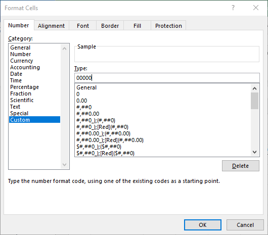
Figure 1. The Number tab of the Format Cells dialog box.

5. In the Type box enter "[Red][>=495]#,##0;[<495]#,##0;;" (without the quote marks).
6. Click OK.

Now any accrued hours that are less than 495 will display normally and anything over that will show up in red. This approach does have some benefits (custom formats don't get messed up like conditional formatting sometimes does), but it means that if your trigger value changes at some point in the future, you'll need to modify the custom format directly.

ExcelTips is your source for cost-effective Microsoft Excel training. This tip (13496) applies to Microsoft Excel 2007, 2010, 2013, 2016, 2019, Excel in Microsoft 365, and 2021.