Please Note: This article is written for users of the following Microsoft Excel versions: 2007 and 2010. If you are using an earlier version (Excel 2003 or earlier), this tip may not work for you. For a version of this tip written specifically for earlier versions of Excel, click here: Formatting the Border of a Legend.
When you create a chart in Excel, the Wizard that you follow may create a chart legend, depending on the type of chart you are creating. Normally, the appearance of the legend will be acceptable for the type of chart you are creating. You have complete control, however, over how the legend appears.
One of the elements you can change is the type of border Excel places around the legend. To change the appearance of the legend's border, follow these steps:
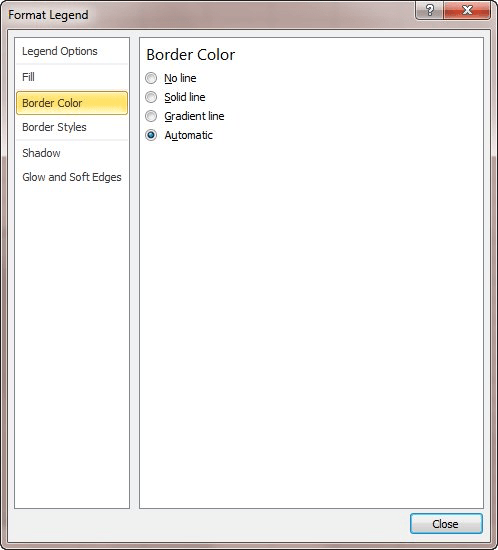
Figure 1. The Format Legend dialog box.
ExcelTips is your source for cost-effective Microsoft Excel training. This tip (6153) applies to Microsoft Excel 2007 and 2010. You can find a version of this tip for the older menu interface of Excel here: Formatting the Border of a Legend.

Dive Deep into Macros! Make Excel do things you thought were impossible, discover techniques you won't find anywhere else, and create powerful automated reports. Bill Jelen and Tracy Syrstad help you instantly visualize information to make it actionable. You�ll find step-by-step instructions, real-world case studies, and 50 workbooks packed with examples and solutions. Check out Microsoft Excel 2019 VBA and Macros today!
Displaying information using charts in Excel is easy and there are a variety of chart styles to choose from. Integrated ...
Discover MoreNeed to move a chart legend to a different place on the chart? It's easy to do using the mouse, as described in this tip.
Discover MoreWhen you create a chart in Excel, the program may automatically add a legend that explains the contents of the chart. In ...
Discover MoreFREE SERVICE: Get tips like this every week in ExcelTips, a free productivity newsletter. Enter your address and click "Subscribe."
2020-04-14 11:29:28
Dave Bonin
This is a late answer for "The Bruce", but I thought some of my special approaches might be useful to others.
I'm often at odds with Excel charting. While it's very powerful, it can also be very constraining in certain situations.
When that happens, I creatively apply other methods Excel provides.
- When Excel can't format axis titles quite the way I want them (perhaps I want to color, italicize or bold part of the title), I turn off the chart axis title and put axis title in the cells behind the chart. By adjusting row heights, column widths and merging cells, I can usually get exactly what I need.
- Ditto for chart titles.
- When I can't get the chart legend the way I want, I create my own. I've used MS Paint to build a chart legend image and then pasted it as a picture over the chart. I've also used text boxes. This can be especially handy when your chart includes a ghost series or two that you don't want in the chart legend. Sometimes, I've used snip to copy Excel's chart legend which I then edited with MS Paint and then pasted as a picture over the chart.
- I've also set up bar charts so that each bar aligns with it's own Excel column or row (column for a vertical bar chart, row for a horizontal bar chart) and then inserted the bar names into the appropriate cells.
- One special note -- when I put legends and titles in cells under a chart, I format the chart area to have no borders and no color. Instead, I color the cells under the chart and apply a suitable border.
By now, some readers may be shaking their heads at these techniques. Admittedly, I don't use them often. But they sure come in handy in those special cases where they're needed. And in my 25 years of using Excel, those special cases have come up pretty often.
2018-01-25 19:03:52
The Bruce
Do you know of a way to format a legend so that the series color dot is larger and placed above the legend text rather than to the left and relatively small as is the standard? (see Figure 1 below)
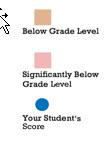
Figure 1. Mock up of what is desired
Got a version of Excel that uses the ribbon interface (Excel 2007 or later)? This site is for you! If you use an earlier version of Excel, visit our ExcelTips site focusing on the menu interface.
FREE SERVICE: Get tips like this every week in ExcelTips, a free productivity newsletter. Enter your address and click "Subscribe."
Copyright © 2026 Sharon Parq Associates, Inc.
 Please Note:
This article is written for users of the following Microsoft Excel versions: 2007 and 2010. If you are using an earlier version (Excel 2003 or earlier), this tip may not work for you. For a version of this tip written specifically for earlier versions of Excel, click here:
Please Note:
This article is written for users of the following Microsoft Excel versions: 2007 and 2010. If you are using an earlier version (Excel 2003 or earlier), this tip may not work for you. For a version of this tip written specifically for earlier versions of Excel, click here:
Comments