Conditionally Formatting for Multiple Date Comparisons

Bev is having a problem setting up a conditional format for some cells. What she wants to do is to format the cells so that if they contain a date before today, they will use a bold red font; if they contain a date after today, they will use a bold green font. Bev cannot get both conditions to work properly.

What is probably happening here is a frustrating artifact of the way that Excel parses the conditions you enter. Follow these steps to see what I mean:

1. Select the range of dates to which you want the conditional format applied.
2. With the Home tab of the ribbon displayed, click the Conditional Formatting option in the Styles group. Excel displays a palette of options related to conditional formatting.
3. Choose Manage Rules. Excel displays the Conditional Formatting Rules Manager dialog box.
4. Click New Rule. Excel displays the New Formatting Rule dialog box.
5. In the Select a Rule Type area at the top of the dialog box, choose Format Only Cells that Contain. (See Figure 1.)



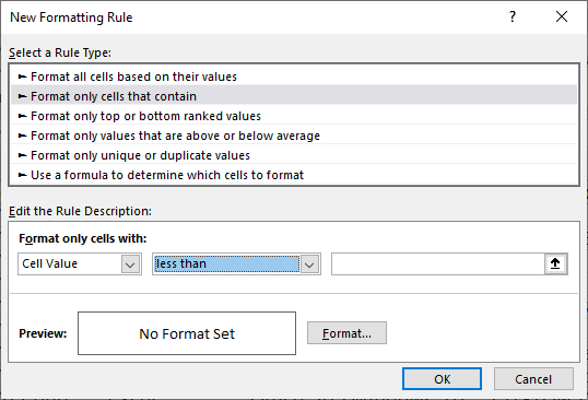
Figure 1. The New Formatting Rule dialog box.

6. In the Edit the Rule Description area, change the second drop-down list to Less Than.
7. In the area just to the right of the drop-down list enter =TODAY().
8. Click Format. Excel displays the Format Cells dialog box. Make sure the Font tab is displayed. Change the formatting for the font to bold red, then close the Format Cells dialog box.
9. Click OK. Excel closes the New Formatting Rule dialog box and shows the rule in the Conditional Formatting Rules Manager dialog box.
10. Click New Rule. Excel again displays the New Formatting Rule dialog box.
11. In the Select a Rule Type area at the top of the dialog box, choose Format Only Cells that Contain.
12. In the Edit the Rule Description area, change the second drop-down list to Greater Than.
13. In the area just to the right of the drop-down list enter =TODAY().
14. Click Format. Excel displays the Format Cells dialog box. Make sure the Font tab is displayed. Change the formatting for the font to bold green, then close the Format Cells dialog box.
15. Click OK. Excel closes the New Formatting Rule dialog box and shows the second rule in the Conditional Formatting Rules Manager dialog box.
16. Click the up and down arrows to move the rules you created to the order in which they should be evaluated.
17. Click OK to close the Conditional Formatting Rules Manager dialog box.

Any dates prior to today will be bold red and any after today will be bold green. If the date is today's date, then it will not be formatted in any particular manner.

ExcelTips is your source for cost-effective Microsoft Excel training. This tip (12929) applies to Microsoft Excel 2007, 2010, 2013, 2016, 2019, and 2021. You can find a version of this tip for the older menu interface of Excel here: Conditionally Formatting for Multiple Date Comparisons.