Contingent Validation Lists

The data validation capabilities in Excel are quite handy, particularly if your worksheets will be used by others. When developing a worksheet, you might wonder if there is a way to make the choices in one cell contingent on what is selected in a different cell. For instance, you may set up the worksheet so that cell A1 uses data validation to select a product from a list of products. You would then like the validation rule in cell B1 to present different validation lists based on the product selected in A1.

The easiest way to accomplish this task is in this manner:

1. Beginning at cell F1, set up a data table. This table will contain your product "matrix." In the first cell of each column, indicate a category name, such as Computers, Televisions, and Recorders.
2. Under each heading in the product matrix, list the various products in the category.
3. Select the headings from the data table, such as F1:H1.
4. Display the Formulas tab of the ribbon.
5. Click the Define Name tool in the Defined Names group. Excel displays the New Name dialog box. (See Figure 1.)



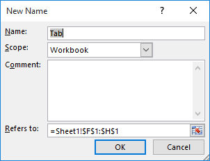
Figure 1. The New Name dialog box.

6. In the Name box, enter a descriptive name, such as Choices.
7. Click OK to add the name and close the dialog box.
8. Select the actual products in column F. Don't select the heading (F1); just select the products under the heading.
9. Again, display the New Name dialog box, as described in steps 4 and 5.
10. In the Name box, enter the same name you used as a heading in that column, such as Computers.
11. Click OK to add the name and close the dialog box.
12. Repeat steps 8 through 11 for the other product columns. In each case, make sure you define the name as the same name used in the column header.
13. Select cell A1.
14. Display the Data tab of the ribbon.
15. 15. Click the Data Validation tool in the Data Tools group. Excel displays the Data Validation dialog box. (See Figure 2.)



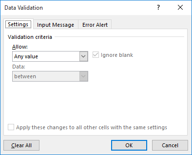
Figure 2. The Data Validation dialog box.

16. Using the Allow drop-down list, choose List.
17. In the Source box, enter an equal sign followed by the name you defined in step 6 (such as =Choices).
18. Click OK.
19. Select cell B1 and again display the Data Validation dialog box as described in step 15.
20. Using the Allow drop-down list, choose List.
21. In the Source box, enter the following: =INDIRECT(A1).
22. Click OK. Excel displays a dialog box asking if you really want to use the rule. (This is because the referenced cell, A1, currently resolves to an error condition.)
23. Click Yes.

That's it. Now, whatever is chosen in cell A1 dictates which list is presented in cell B1.

ExcelTips is your source for cost-effective Microsoft Excel training. This tip (11943) applies to Microsoft Excel 2007, 2010, 2013, 2016, 2019, and Excel in Microsoft 365. You can find a version of this tip for the older menu interface of Excel here: Contingent Validation Lists.