Disabling #SPILL! Errors

Jan's company recently upgraded to Office 365 ProPlus. With it came a #SPILL! error when using VLOOKUP, which he uses a LOT. He is now unable to use VLOOKUP with a filter. Jan knows it would be easy to sort and/or to remove the #N/A that came from the previous VLOOKUP, but this error is causing him a lot of extra time and effort. He wonders if there is a way to turn this "feature" off.

In the very near past, Microsoft changed how it calculates worksheets. This was a HUGE change, and you may have read about it elsewhere. Here's one article that provides some great information on the change:

https://exceljet.net/dynamic-array-formulas-in-excel

The article is rather long; you'll want to set aside some time to digest the information it contains. If you create lots of formulas in Excel, you'll want to do so, though—the change to the program means you must understand it, eventually.

Essentially, Microsoft did away with the concept of array functions (though they will still work), instead allowing almost all functions, including VLOOKUP, to return an array of values. If the array of returned values won't fit in the available space, you get the new #SPILL! error.

Quite honestly, the answer isn't to disable #SPILL! errors; there really is no way to do so. The answer is to understand what Excel is now doing as it calculates and then modify your formulas accordingly.

Let's look at an example. Let's say you have a worksheet that lists items and their prices in a simple two-column set of data. Then, to the right of this, you enter some items and use a VLOOKUP function to return the prices associated with each of those items. When you open this workbook in an older version of Excel (2019 or earlier) you get great results. (See Figure 1.)

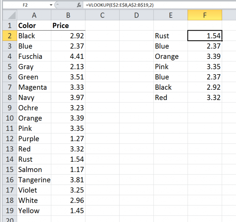
Figure 1. A simple VLOOKUP formula in Excel 2010.

This screen shot was taken using an Excel 2010 system, but it would work the same if you looked at it in Excel 2016 or even Excel 2019. Note in this example that the VLOOKUP formula in cell F2 (shown in the Formula bar because cell F2 is selected) is copied down to the range F2:F8. You get the desired results because the VLOOKUP function returns a single value from the table.

Now, let's look at what happens if you create the same workbook, using the same formulas, in the version of Excel provided with Office 365. In this case you will see errors. (See Figure 2.)

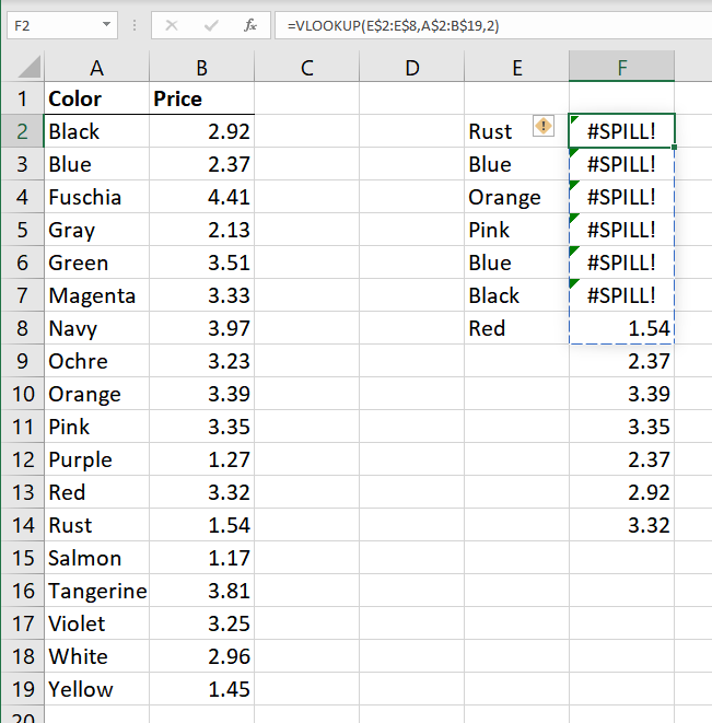
Figure 2. The same simple VLOOKUP formula in the latest version of Excel.

Notice the #SPILL! errors. This error occurs because the VLOOKUP formula can now return more than a single value. In fact, when you use a range of cells in the very first parameter for VLOOKUP, it will now return a value for each cell in that range. Thus, using the range E2:E8 for the first parameter means that VLOOKUP returns 7 values. In other words, it automatically returns an array of values. If those values cannot all be displayed, then you get the #SPILL! error. That is why you are seeing the #SPILL! error in cells F2:F7; there are things below them that stop all the values returned in those formulas from being displayed. You don't see the error in cell F8 because there is nothing below that cell stopping the display.

So, how do you fix this? There are actually three ways you can fix it. In this particular example, the easiest way would be to simply delete everything in cells F3:F8. This allows the formula in cell F2 to "spill" correctly to the rest of the cells below it.

The second approach would be to change the formula in cell F2, so it looks like this:

=VLOOKUP(@E$2:E$8,A$2:B$19,2)

Notice the use of the @ symbol just before the first parameter. This tells Excel that you want the VLOOKUP formula to return just a single value. The other way to adjust the formula would be to make it look like this in cell F2:

=VLOOKUP(E2,A$2:B$19,2)

Now you can copy either formula down from cell F2 into the full range of F2:F8 and you won't have a problem. Why? Because (again) VLOOKUP in these instances is returning only a single value, not an array of values.

The upshot is that the best way to change your formulas is to either (1) make sure there is nothing blocking the display of the full array of values you are requesting VLOOKUP to return or (2) modify the first parameter so that it references just a single cell.

ExcelTips is your source for cost-effective Microsoft Excel training. This tip (13750) applies to Microsoft Excel Excel in Microsoft 365.