Please Note: This article is written for users of the following Microsoft Excel versions: 2007, 2010, 2013, 2016, 2019, and 2021. If you are using an earlier version (Excel 2003 or earlier), this tip may not work for you. For a version of this tip written specifically for earlier versions of Excel, click here: Shortcut for Viewing Formulas.
You probably already know how to display the formulas in cells rather than the results of those formulas, right? If you're like most people, you follow these steps:
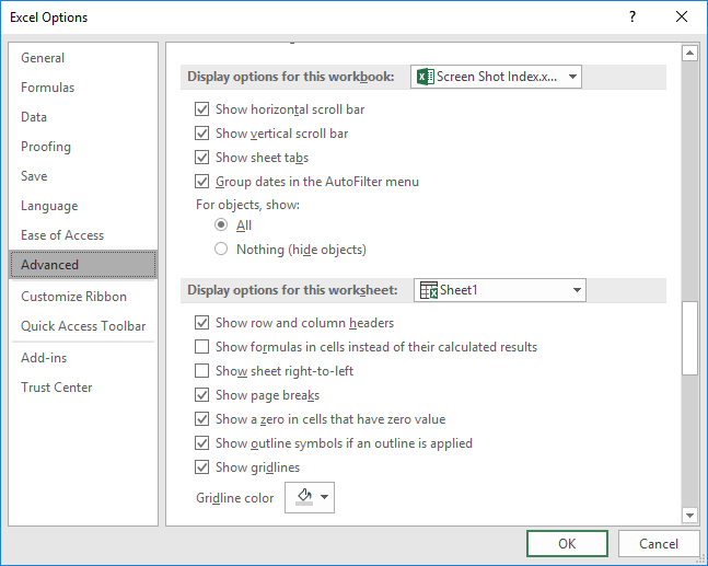
Figure 1. The Display Options for a worksheet.
A much faster way to get the same result is to simply press Ctrl+`. (That's hold down the Ctrl key while you press the accent grave, which is the backwards apostrophe just to the left of the 1 key and above the Tab key.) The shortcut is a toggle, which means that you can press it repeatedly to switch between the display of formulas and results.
ExcelTips is your source for cost-effective Microsoft Excel training. This tip (6198) applies to Microsoft Excel 2007, 2010, 2013, 2016, 2019, and 2021. You can find a version of this tip for the older menu interface of Excel here: Shortcut for Viewing Formulas.

Dive Deep into Macros! Make Excel do things you thought were impossible, discover techniques you won't find anywhere else, and create powerful automated reports. Bill Jelen and Tracy Syrstad help you instantly visualize information to make it actionable. You�ll find step-by-step instructions, real-world case studies, and 50 workbooks packed with examples and solutions. Check out Microsoft Excel 2019 VBA and Macros today!
Got a list of data from which you want to delete duplicates? There are a couple of techniques you can use to get rid of ...
Discover MoreIf you keep a lot of data in Excel, you may be interested in figuring out when that data surpasses a threshold. This tip ...
Discover MoreNeed to count the number of W (win) or L (loss) characters in a range of cells? You can develop a number of formulaic ...
Discover MoreFREE SERVICE: Get tips like this every week in ExcelTips, a free productivity newsletter. Enter your address and click "Subscribe."
2022-12-21 11:29:45
J. Woolley
The following function mentioned in Peter's comment below will also return an array of formulas when Target is a range of cells on any worksheet:
=FORMULATEXT(Target)
In this case the returned array will be the same size as Target; cells that are blank or contain constants will be marked #N/A.
2022-12-20 14:40:57
J. Woolley
My Excel Toolbox includes the following dynamic array function to return all non-blank formulas with optional values from a Target range of cells on any worksheet:
=ListFormulas(Target,[WithValues],[SkipConstants],[SkipHeader])
Expect 2 columns (Cell, Formula) or 3 columns (Cell, Formula, Value) and N rows (plus header). When SkipConstants is TRUE only formulas that begin with = will be returned.
My Excel Toolbox's SpillArray function simulates a dynamic array in older versions of Excel:
=SpillArray(ListFormulas(...))
See UseSpillArray.pdf at https://sites.google.com/view/MyExcelToolbox
2021-05-11 05:25:33
Peter
I like the options for invoking formulas quickly, but I am not a fan of the all or nothing mode of operation.
I have recently discovered =FORMULATEXT(), which gives me the ability to review formulae and calculated results at the same time.
2021-05-10 07:52:36
Russell Stainer
Another way to do it, is to go to the 'Formulas' tab in the ribbon, go to the 'Formula Auditing' group, and toggle 'Show Formulas'. If you right-click it, you can also add it to the Quick Access Toolbar.
Got a version of Excel that uses the ribbon interface (Excel 2007 or later)? This site is for you! If you use an earlier version of Excel, visit our ExcelTips site focusing on the menu interface.
FREE SERVICE: Get tips like this every week in ExcelTips, a free productivity newsletter. Enter your address and click "Subscribe."
Copyright © 2026 Sharon Parq Associates, Inc.
 Please Note:
This article is written for users of the following Microsoft Excel versions: 2007, 2010, 2013, 2016, 2019, and 2021. If you are using an earlier version (Excel 2003 or earlier), this tip may not work for you. For a version of this tip written specifically for earlier versions of Excel, click here:
Please Note:
This article is written for users of the following Microsoft Excel versions: 2007, 2010, 2013, 2016, 2019, and 2021. If you are using an earlier version (Excel 2003 or earlier), this tip may not work for you. For a version of this tip written specifically for earlier versions of Excel, click here:
Comments