Ben has a worksheet that contains text values in column A. He needs to calculate the number of cells that contain the word "priority." He knows how to do the count if "priority" is the only word in a cell, but that's not always the case. Most of the time the word is within a sentence or a sentence fragment contained in a cell. Ben doesn't need the number of times the word appears (it may appear twice in some cells), but only the number of cells that contain the word at least once.
There are several ways you can accomplish this task. There are some questions that should be answered, though, before choosing a formula. For instance, do you want the count to be case sensitive? Do you only want to count "priority" when it is a whole word, or do you want to count when it is part of another word ("apriority")? What version of Excel is being used?
An easy way to count instances and take most of these questions into account is to use Find and Replace. Select the range of cells for which you want a count and use the Find tool (Ctrl+F) to search for "priority." Make sure, in the Find and Replace dialog box, you set the Look In drop-down list to Values and check the Match Case check box as desired. When you click on Find All, the dialog box reports the number of occurrences in the selected range—the number of cells in which "priority" appears.
If you want to use the count in a formula, then you need to use a formula to derive the count. The easiest approach is to use the COUNTIF function with a search string that includes wildcards:
=COUNTIF(A:A,"*priority*")
This counts the number of cells in column A that contain the word "priority" either by itself or surrounded by any number of characters. The matching is not case sensitive, so it will match "priority" or "Priority" or "PRIORITY" just the same. Here's a variation that will return the same result:
=COUNT(SEARCH("priority",A:A))
If you want the count to be case sensitive, then you can use a formula that is a bit more complex:
=SUM(N(A1:A9<>SUBSTITUTE(A1:A9,"Priority",)))
Simply put, within the quote marks, the mix of upper- and lowercase you want to use.
If you want to only count "priority" when it is a whole word, then you are going to need to use a formula that relies on the REGEXTEST function, which is available in Excel XXX and Excel in Microsoft 365. This variation is case sensitive:
=SUM(--REGEXTEST(A:A,"\bpriority\b"))
By default, REGEXTEST pays attention to case. You can make the formula case insensitive by adding an additional parameter to the end of the function:
=SUM(--REGEXTEST(A:A,"\bpriority\b",1))
ExcelTips is your source for cost-effective Microsoft Excel training. This tip (11109) applies to Microsoft Excel 2007, 2010, 2013, 2016, 2019, 2021, 2024, and Excel in Microsoft 365.

Program Successfully in Excel! This guide will provide you with all the information you need to automate any task in Excel and save time and effort. Learn how to extend Excel's functionality with VBA to create solutions not possible with the standard features. Includes latest information for Excel 2024 and Microsoft 365. Check out Mastering Excel VBA Programming today!
Define a named range today and you may want to change the definition at some future point. It's rather easy to do, as ...
Discover MoreWhen you construct a formula and click on a cell in a different workbook, an absolute reference to that cell is placed in ...
Discover MoreSearching for a value using Excel's Find tool is easy; searching for that same value using a formula or a macro is more ...
Discover MoreFREE SERVICE: Get tips like this every week in ExcelTips, a free productivity newsletter. Enter your address and click "Subscribe."
2025-08-17 01:58:56
Alex Blakenburg
Oops bad example, if your data starts at A1 you could use A:.A.
If your data starts further down the sheet you will most likely benefit from setting a row range A5:.A100000.
2025-08-17 01:55:02
Alex Blakenburg
@RaySMc - In order of appearance above.
=COUNTIF(A:A,"*" & $D$2 & "*")
=COUNT(SEARCH($D$2,A:A))
=SUM(N(A1:A9<>SUBSTITUTE(A1:A9,$D$2,))) Case Sensitive
=SUM(--REGEXTEST(A:A,"\b" & $D$2 & "\b")) Case Sensitive
=SUM(--REGEXTEST(A:A,"\b" & $D$2 & "\b",1))
Note: the 2 Regex versions with whole column reference are performance killers. If you have Regex you will have TrimRange so instead of A:A use something like A1:.A100000 (there is a period before the 2nd A which will drop unused rows and shrink the range)
2025-08-16 19:11:20
RaySMc
In any of the examples given for this tip, how can a cell reference (e.g., D2) containing the text string of interest be used in place of "priority"?
2025-08-16 12:08:46
J. Woolley
@jamies
The RegEx metacharacter \b matches anything that is not a \w word character, and a \w word character is equivalent to the set [A-Za-z0-9_].
If your version of Excel doesn't include REGEXTEST, My Excel Toolbox has the equivalent function IsRegEx.
See https://sites.google.com/view/MyExcelToolbox/
2025-08-16 11:37:55
J. Woolley
@Hazel Kohler
1. Select the cells you want to format
2. Choose Home > Conditional Formatting > New Rule (Alt+H,L,N) to open the New Formatting Rule dialog
3. Pick "Use a formula..."
4. Enter this formula: =NOT(ISERROR(SEARCH("priority", A1)))
5. Click Format... to define the conditional format
6. Click OK
The formula in step 4 assumes your trigger is "priority" and the range you selected in step 1 begins with cell A1; adjust the formula to suit your requirement.
(see Figure 1 below)
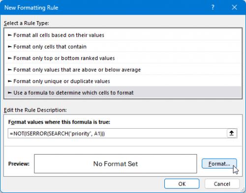
Figure 1.
2025-08-16 10:59:24
jamies
Maybe also worth checking for trailing punctuation, and maybe also leading braces, brackets, apostrophe and quote and even "newline - remembering that excel will bound text as well as use a leading apostrophe or caret ^ to indicate data entered is to be stored as "text" in a cell, with the possibility that the user has added a leading ' to force the entry to be held as "text" and not converted as if it was a date, or floating point
-
note
Lotus123 used apostrophe (') for left-aligned text, double quote (") for right-aligned text, and caret (^) for centred text.
That can cause some confusion with some Excel settings.
sort of like entering a date of 29th February 1900 - that is accepted as a date - with the day after being 1st March !
or calculating the day before the 1st March 1900 -
2025-08-16 09:34:38
Hazel Kohler
I have a related requirement - to use a character string that could be anywhere (or not) in a cell as the trigger for conditional formatting. Any suggestions gratefully received!
Got a version of Excel that uses the ribbon interface (Excel 2007 or later)? This site is for you! If you use an earlier version of Excel, visit our ExcelTips site focusing on the menu interface.
FREE SERVICE: Get tips like this every week in ExcelTips, a free productivity newsletter. Enter your address and click "Subscribe."
Copyright © 2026 Sharon Parq Associates, Inc.
Comments