Please Note: This article is written for users of the following Microsoft Excel versions: 2007, 2010, 2013, 2016, 2019, 2021, and Excel in Microsoft 365. If you are using an earlier version (Excel 2003 or earlier), this tip may not work for you. For a version of this tip written specifically for earlier versions of Excel, click here: Conditional Format that Checks for Data Type.
Written by Allen Wyatt (last updated May 27, 2023)
This tip applies to Excel 2007, 2010, 2013, 2016, 2019, 2021, and Excel in Microsoft 365
Joshua is trying to establish a conditional format that will alert a user that text data has been entered into a cell intended for numerical data or when numerical data has been input into a cell intended for text data.
A conditional format can be used to draw attention to when an improper value (text or numeric) has been entered in a cell, but a more robust approach might be to prohibit the improper value from being entered in the first place. This can be done with the data validation capabilities of Excel. These capabilities have been discussed, in detail, in other ExcelTips; more information can be found here:
http://excelribbon.tips.net/C0786_Data_Validation.html
Using data validation you can specify the type and range of data permitted in a cell, along with how stringently you want that specification followed. If you prefer to not use data validation for some reason, you can set up a conditional format that will verify if the information placed in a cell is of the data type you want. Follow these steps:
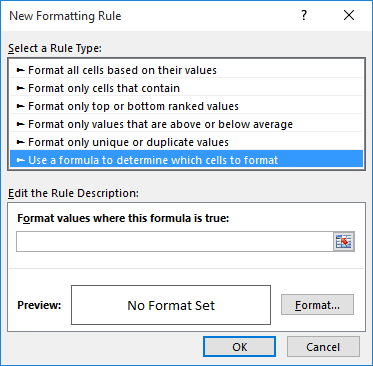
Figure 1. The New Formatting Rule dialog box.
     =ISTEXT(A1)
     =ISNUMBER(A1)
ExcelTips is your source for cost-effective Microsoft Excel training. This tip (7073) applies to Microsoft Excel 2007, 2010, 2013, 2016, 2019, 2021, and Excel in Microsoft 365. You can find a version of this tip for the older menu interface of Excel here: Conditional Format that Checks for Data Type.

Professional Development Guidance! Four world-class developers offer start-to-finish guidance for building powerful, robust, and secure applications with Excel. The authors show how to consistently make the right design decisions and make the most of Excel's powerful features. Check out Professional Excel Development today!
Conditional formatting is a great tool for changing how your data looks based on the data itself. Excel won't allow you ...
Discover MoreConditional formatting rules can be used to adjust the way in which information is displayed in Excel, such as the text ...
Discover MoreWhen you apply conditional formatting, you are not limited to using a single condition. Indeed, you can set up multiple ...
Discover MoreFREE SERVICE: Get tips like this every week in ExcelTips, a free productivity newsletter. Enter your address and click "Subscribe."
There are currently no comments for this tip. (Be the first to leave your comment—just use the simple form above!)
Got a version of Excel that uses the ribbon interface (Excel 2007 or later)? This site is for you! If you use an earlier version of Excel, visit our ExcelTips site focusing on the menu interface.
FREE SERVICE: Get tips like this every week in ExcelTips, a free productivity newsletter. Enter your address and click "Subscribe."
Copyright © 2025 Sharon Parq Associates, Inc.
 Please Note:
This article is written for users of the following Microsoft Excel versions: 2007, 2010, 2013, 2016, 2019, 2021, and Excel in Microsoft 365. If you are using an earlier version (Excel 2003 or earlier), this tip may not work for you. For a version of this tip written specifically for earlier versions of Excel, click here:
Please Note:
This article is written for users of the following Microsoft Excel versions: 2007, 2010, 2013, 2016, 2019, 2021, and Excel in Microsoft 365. If you are using an earlier version (Excel 2003 or earlier), this tip may not work for you. For a version of this tip written specifically for earlier versions of Excel, click here:
Comments