Conditional Formats that Distinguish Blanks and Zeroes

Let's say that you routinely import information from another program into Excel. The information contains numeric values, but it can also contain blanks. You might want to use a conditional format on the imported information to highlight any zero values. The problem is, if you just add a conditional format that highlights the cells to see if they are zero, then the condition will also highlight any cells that are blank, since they contain a "zero" value, as well.

There are several different solutions to this predicament. One solution is to apply a conditional format that uses two conditions. The first condition checks for the blanks, and the second checks for zero values. The condition that checks for blanks doesn't need to adjust any formatting, but the one that checks for zero values can. This works because if the first condition is satisfied (the cell is blank), the second condition is never tested. Do the following:

1. Select the range you want conditionally formatted. (For this example, I'll assume that you've selected the range A2:A99.)
2. With the Home tab of the ribbon displayed, click the Conditional Formatting option in the Styles group. Excel displays a palette of options related to conditional formatting.
3. Click Manage Rules. Excel displays the Conditional Formatting Rules Manager dialog box.
4. Click New Rule. Excel displays the New Formatting Rule dialog box.
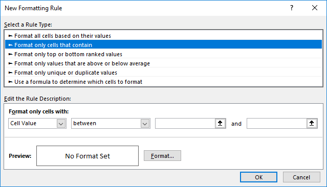
5. In the Select a Rule Type area at the top of the dialog box, choose Format Only Cells That Contain. (See Figure 1.)



Figure 1. The New Formatting Rule dialog box.

6. Using the first drop-down list for the rule, choose Blanks.
7. Click OK. Excel closes the New Formatting Rule dialog box and again displays the Conditional Formatting Rules Manager dialog box, this time with your new rule visible. (Note that you didn't specify any formatting for this rule; that's fine.)
8. Make sure the Stop If True check box is selected for the rule.
9. Click New Rule. Excel again displays the New Formatting Rule dialog box.
10. In the Select a Rule Type area at the top of the dialog box, choose Format Only Cells That Contain.
11. Using the first drop-down list for the rule, choose Cell Value.
12. Using the second drop-down list for the rule, choose Equal To.
13. In the value box for Condition 2, enter 0.
14. Click the Format button. Excel displays the Format Cells dialog box.
15. Use the controls in the dialog box to modify the formatting, as desired.
16. Click OK to close the Format Cells dialog box.
17. Click OK to close the New Formatting Rule dialog box. Excel again displays the Conditional Formatting Rules Manager, and the rule you just defined is the first one in the list. (It should also be selected.)
18. Click the down arrow to move the rule you just created to the second position in the list of rules.
19. Click OK to close the Conditional Formatting Rules Manager dialog box. The formatting is applied to the range of cells you selected in step 1.

Another solution is to combine your two conditions into a single condition. Follow these steps:

1. Select the range you want conditionally formatted. (For this example, I'll assume that you've selected the range A2:A99.)
2. With the Home tab of the ribbon displayed, click the Conditional Formatting option in the Styles group. Excel displays a palette of options related to conditional formatting.
3. Click New Rule. Excel displays the New Formatting Rule dialog box.
4. In the Select a Rule Type area at the top of the dialog box, choose Use a Formula To Determine Which Cells to Format.
5. In the formula box enter the formula =AND(A2=0,A2<>"").
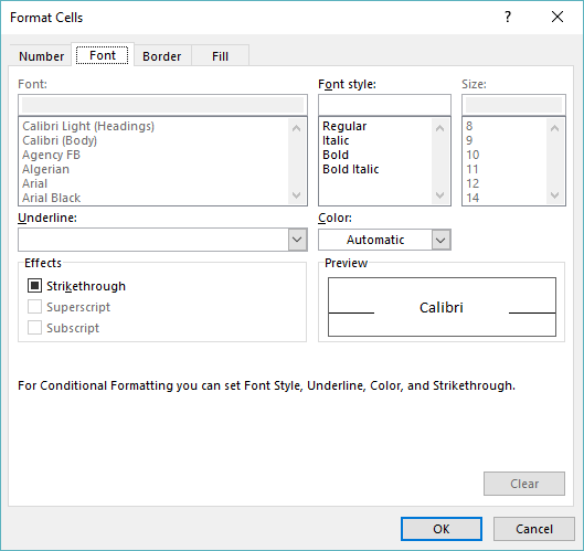
6. Click the Format button. Excel displays the Format Cells dialog box. (See Figure 2.)



Figure 2. The Format Cells dialog box.

7. Use the controls in the dialog box to modify the formatting, as desired.
8. Click OK to close the Format Cells dialog box.
9. Click OK to close the New Formatting Rule dialog box. The formatting is applied to the range of cells you selected in step 1.

The formula used in step 5 checks to make sure that the value is 0 and that the cell is not blank. The AND function makes sure that only when both criteria are satisfied will the formula return True and the format be applied.

There are any number of other formulas that could also be used. For instance, each of the following formulas could be substituted in step 5:

• =AND(COUNT(A2)=1,A2=0)
• =AND(A2=0,NOT(ISBLANK(A2)))
• =AND(A2=0,LEN(A2)>0)
• =NOT(ISBLANK(A2))*(A2=0)

If you wanted an even faster way to highlight zero values while ignoring blanks, you might consider using a macro. The macro would be faster because you could just import and run it; you don't have to select a range of cells and enter the formula (or formulas) for the conditional formatting. The following macro is an example of one you could use:

Sub FormatRed()
    TotalRows = 5000
    ColNum = 1

    For i = 1 To Cells(TotalRows, ColNum).End(xlUp).Row
        Cells(i, ColNum).Interior.ColorIndex = xlAutomatic
        If IsNumeric(Cells(i, ColNum).Value) Then
            If Cells(i, ColNum).Value = 0 Then
                Cells(i, ColNum).Interior.ColorIndex = 3
            End If
        End If
    Next
End Sub

The macro checks the cells in column A. (It checks the cells in rows 1 through 5,000; you can modify this, if desired.) If the cell contains a numeric value and that value is zero, then the cell is filled with red. If the cell contains something else, then the cell is set back to its normal color.

For more ideas about conditional formatting and blank cells, see this site:

https://www.ablebits.com/office-addins-blog/excel-conditional-formatting-blank-cells/

ExcelTips is your source for cost-effective Microsoft Excel training. This tip (7131) applies to Microsoft Excel 2007, 2010, 2013, 2016, 2019, Excel in Microsoft 365, and 2021. You can find a version of this tip for the older menu interface of Excel here: Conditional Formats that Distinguish Blanks and Zeroes.