Getting a Count of Unique Names

John has a worksheet that he uses for registration of attendees at a conference. Column A has a list of each person attending, and column B has the company represented by each attendee. Each company can have multiple people attend. John can easily figure out how many individuals are coming to the conference; it is simply the number of rows in column A (minus any header rows). The more difficult task is to determine how many companies are going to be represented at the conference.

There are a few ways to determine the desired count. If you are using Excel 2021 or the version of Excel in Microsoft 365, then you can rely on a couple of great new functions. First, you can use the UNIQUE function to get a list of all of the unique company names. Combine it with the SORT function, and you can see the companies in a sorted order that allows you to quickly spot any misspellings:

=SORT(UNIQUE(B2:B50))

Or, if you prefer to have just a count of unique companies (like John wants), then you can use this formula:

=COUNTA(UNIQUE(B2:B50))

If you are using an older version of Excel, then getting the answer you want can be a bit more convoluted. If there are no blank cells in column B, you can use an array formula (entered by Ctrl+Shift+Enter) such as the following:

=SUM(1/COUNTIF(B2:B50,B2:B50))

If there are blanks in the range (B2:B50 in this case), then the array formula will return a #DIV/0! error. If that is the case, the array formula needs to be changed to the following:

=SUM(IF(FREQUENCY(IF(LEN(B2:B50)>0,MATCH(B2:B50,B1:B50,0),
""),IF(LEN(B2:B50)>0,MATCH(B2:B50,B2:B50,0),""))>0,1))

If you prefer to not use an array formula, you can add regular formulas to column C to do the count. First, sort the table of data by the contents of column B. That way the data will be in company order. Then add a formula such as the following to cell C2 (assuming you have a header in row 1):

=IF(B2<>B3,1,0)

Copy the formula down through all the rest of the cells in column C, and then do a sum on the column. The sum represents the number of unique companies attending, since a 1 only appears in column C when the company name changes.

Of course, if you need to find the names of all the companies represented at the conference, you can use Excel's filtering capabilities. Follow these steps:

1. Sort the data by column B, the company names.
2. Select all the cells containing data (including the header cell) in column B.
3. Display the Data tab of the ribbon.
4. Click the Advanced tool, in the Sort & Filter group. Excel displays the Advanced Filter dialog box. (See Figure 1.)



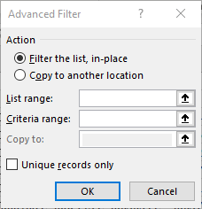
Figure 1. The Advanced Filter dialog box.

5. Make sure the Copy to Another Location radio button is selected.
6. Make sure the Unique Records Only check box is selected.
7. With the insertion point in the Copy To box, click on a blank cell, such as E1. (This is where the list of companies will be copied to.)
8. Click OK. Excel copies the unique company names from the original list to column E.

You now can easily see how many companies are being represented, along with who those companies are.

Finally, you can also use a simple PivotTable to figure out the number of companies. Create the PivotTable based on your data, using the company name column as a row label. This will give you the list of unique company names, which can easily be counted.

ExcelTips is your source for cost-effective Microsoft Excel training. This tip (7562) applies to Microsoft Excel 2007, 2010, 2013, 2016, 2019, 2021, and Excel in Microsoft 365. You can find a version of this tip for the older menu interface of Excel here: Getting a Count of Unique Names.