Password Protecting Specific Columns in a Worksheet

Mary Lou wonders if there is a way she can password protect certain columns in a shared workbook. The workbook has only a single worksheet, and she needs to protect columns E and J so they cannot be changed, unless the user knows a particular password.

The traditional way to approach this challenge is to follow these steps:

1. Select all the cells in your worksheet. (Pressing Ctrl+A will do the trick.)
2. Press Ctrl+Shift+F. Excel displays the Format Cells dialog box.
3. Make sure the Protection tab is displayed. (See Figure 1.)



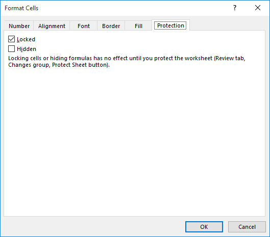
Figure 1. The Protection tab of the Format Cells dialog box.

4. Make sure the Locked check box is cleared. (You may need to click it a few times to get it actually cleared.) This removes protection from all the cells in the worksheet.
5. Click OK to close the Format Cells dialog box.
6. Select column E.
7. Press Ctrl+Shift+F. Excel again displays the Format Cells dialog box.
8. Again make sure the Protection tab is displayed.
9. Make sure the Locked check box is selected. This protects the cells that are currently selected.
10. Click OK to close the Format Cells dialog box.
11. Select column J and repeat steps 7 through 10.
12. Display the Review tab of the ribbon.
13. Click the Protect Sheet tool. Excel displays the Protect Sheet dialog box. (See Figure 2.)



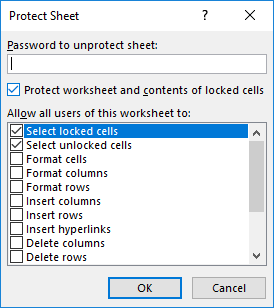
Figure 2. The Protect Sheet dialog box.

14. Make sure the top check box (Protect Worksheet and Contents of Locked Cells) is selected.
15. Enter a password in the appropriate place.
16. Use the check boxes to fine tune how you want protection applied.
17. Click OK. You are again asked to enter the password.
18. Enter the password you used in step 15 a second time. Your worksheet is now protected.

The result of going through all these steps is that the cells in columns E and J cannot be changed. If someone knows the password you used in step 15, however, they can unprotect the worksheet (the proper control is on the Review tab of the ribbon) and make any changes they want. If someone does make changes in this way, they will need to reapply the protection (steps 12 through 17) prior to saving the workbook. If they don't, then the next time the workbook is open, the worksheet remains unprotected and anyone can change the contents of columns E and J.

As I said, the above represents the traditional way to approach the problem. There are non-traditional ways you can use, as well. For instance, you might rethink how your data is put together and, perhaps, move the contents of columns E and J to another worksheet or even to another workbook. You can then protect that information and simply reference it within the current worksheet.

A third approach is to use a tool introduced with the release of Excel 2010. This new tool, which allows you to password-protect ranges of cells, requires a variation on the steps presented earlier in this tip. The steps will be many, but it does provide for a more flexible way of dealing with the protection issue. Here is the variation that includes use of the new tool:

1. Select all the cells in your worksheet. (Pressing Ctrl+A will do the trick.)
2. Press Ctrl+Shift+F. Excel displays the Format Cells dialog box.
3. Make sure the Protection tab is displayed.
4. Make sure the Locked check box is cleared. (You may need to click it a few times to get it actually cleared.) This removes protection from all the cells in the worksheet.
5. Click OK to close the Format Cells dialog box.
6. Select column E.
7. Press Ctrl+Shift+F. Excel again displays the Format Cells dialog box.
8. Again make sure the Protection tab is displayed.
9. Make sure the Locked check box is selected. This protects the cells that are currently selected.
10. Click OK to close the Format Cells dialog box.
11. Select column J and repeat steps 7 through 10.
12. Display the Review tab of the ribbon.
13. Click Allow Users to Edit Ranges. (Click Allow Edit Ranges if you are using Excel in Office 365, Excel 2019, or Excel 2021.) Excel displays the Allow Users to Edit Ranges dialog box. (See Figure 3.)



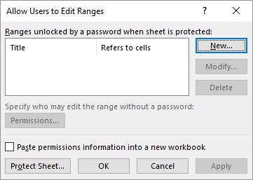
Figure 3. The Allow Users to Edit Ranges dialog box.

14. Click the New button. Excel displays the New Range dialog box. (See Figure 4.)



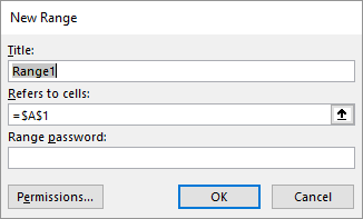
Figure 4. The New Range dialog box.

15. In the Title box, enter the name you want to use for this range. (The title isn't particularly important. Use something that is meaningful to you.)
16. In the Refers to Cells box, enter the following: =$E:$E,$J:$J
17. In the Range Password box, enter the password you want to give to those who should be able to edit columns E and J.
18. Click on OK. You are again asked to enter the password.
19. Enter the password you used in step 17 a second time. The range now appears in the Allow Users to Edit Ranges dialog box.
20. Click OK to close the Allow Users to Edit Ranges dialog box.
21. Click the Protect Sheet tool. Excel displays the Protect Sheet dialog box.
22. Make sure the top check box (Protect Worksheet and Contents of Locked Cells) is selected.
23. Enter a password in the appropriate place. This should not be the same password you used in step 17 and step 19; it should be different.
24. Use the check boxes to fine tune how you want protection applied.
25. Click OK. You are again asked to enter the password.
26. Enter the password you used in step 23 a second time. Your worksheet is now protected.

The advantage to this approach is that you have two levels of passwords—one for the range (columns E and J) and one for the worksheet as a whole. As someone is using a worksheet protected in this manner, when they try to modify a cell in columns E or J, they are asked for a password. If they supply the correct password (this is the one that you specified in steps 17 and 19), then they can edit anything they want in columns E and J. When the workbook is saved, exited, and reopened, then the protection is automatically reset and columns E and J can again only be edited if the password is known—there is no need for the user to explicitly "reprotect" the worksheet before saving. Plus, you never have to give out the password that you used to protect the entire worksheet.

ExcelTips is your source for cost-effective Microsoft Excel training. This tip (8388) applies to Microsoft Excel 2007, 2010, 2013, 2016, 2019, Excel in Microsoft 365, and 2021.