Changing the Color of a Cell Border

You probably already know that Excel allows you to add borders to your cells. This is handy for separating different pieces of information within the same data table and for, well, just making your data look better.

You are not limited to black borders, however. You can specify different colors for your borders by following these steps:

1. Select the cells whose border colors you want to change.
2. Make sure the Home tab of the ribbon is displayed.
3. In the Font group, click the down-arrow next to the Borders tool. You'll see a list of borders you can apply to the cell.
4. Click the More Borders option at the bottom of the list. Excel displays the Border tab of the Format Cells dialog box. (See Figure 1.)



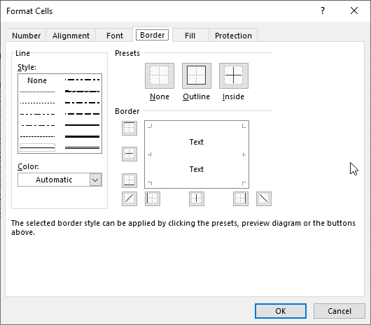
Figure 1. The Border tab of the Format Cells dialog box.

5. Using the Color drop-down list, specify a color you want to use for borders.
6. Using the controls in the dialog box, specify the borders for the cell as you normally would.
7. Click on OK.

Just as you can specify a different border type for each side of a cell, you can also specify a different border color for each side of the cell. Just make sure you pick the color you want used before you click on the side of the cell where you want that color used.

Another way you can change the border color is to use the border drawing tools Excel provides. Just display the Home tab of the ribbon and then click the down-arrow next to the Borders tool (in the Font group). Excel displays a whole bunch of choices for applying borders. (See Figure 2.)

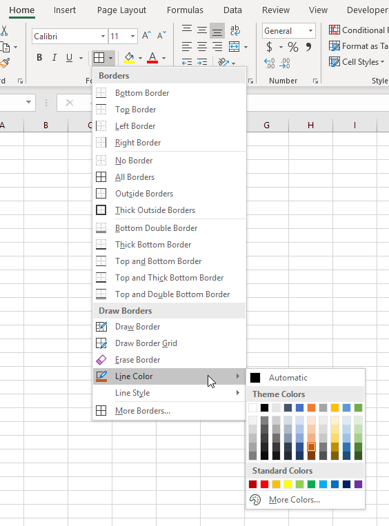
Figure 2. Drawing using a border color.

The option you are interested in is the Line Color option. Hover over it, and you'll see a palette of colors you can choose. Pick the color you want, and Excel kicks into border-drawing mode. (You can tell because the mouse pointer changes to a small pencil shape.) Move near the border you want, hold down the mouse button, and drag the mouse. The border is drawn on the cells as you specify. When you press Esc to exit border-drawing mode, any borders you subsequently apply (by whatever means) are applied in the same color you selected.

ExcelTips is your source for cost-effective Microsoft Excel training. This tip (8773) applies to Microsoft Excel 2007, 2010, 2013, 2016, 2019, and 2021. You can find a version of this tip for the older menu interface of Excel here: Changing the Color of a Cell Border.