Please Note: This article is written for users of the following Microsoft Excel versions: 2007 and 2010. If you are using an earlier version (Excel 2003 or earlier), this tip may not work for you. For a version of this tip written specifically for earlier versions of Excel, click here: Automatically Sorting as You Enter Information.
Pat wonders if there is a way to automatically sort every time she adds new data to a worksheet. Pat thinks it would be great, for instance, that when she adds a new name to a list of names that the names are automatically sorted to always be in order.
The only way that this can be done is by using a macro that is triggered whenever something new is entered in the worksheet. You can, for instance, add a macro to the code for a worksheet that is triggered when something in the worksheet changes. (You can view the code window by right-clicking the worksheet tab and choosing View Code from the resulting Context menu.) The following is an example of one such simple macro:
Private Sub Worksheet_Change(ByVal Target As Range)
    On Error Resume Next
    Range("A1").Sort Key1:=Range("A2"), _
      Order1:=xlAscending, Header:=xlYes, _
      OrderCustom:=1, MatchCase:=False, _
      Orientation:=xlTopToBottom
End Sub
The macro assumes that you want to sort on the data in column A and that there is a header in cell A1. If the names are in a different column, just change the cell A2 reference to a different column, such as B2, C2, etc.
Of course, sorting anytime that any change is made can be bothersome. You might want to limit when the sorting is done so that it only occurs when changes are made to a specific portion of your data. The following version of the macro sorts the data only when a change is made in column A.
Private Sub Worksheet_Change(ByVal Target As Range)
    On Error Resume Next
    If Not Intersect(Target, Range("A:A")) Is Nothing Then
        Range("A1").Sort Key1:=Range("A2"), _
          Order1:=xlAscending, Header:=xlYes, _
          OrderCustom:=1, MatchCase:=False, _
          Orientation:=xlTopToBottom
    End If
End Sub
There are some drawbacks to using a macro to automatically sort your data. First, since you are using a macro to sort, the operation is essentially "final." In other words, after the sorting you can't use Ctrl+Z to undo the operation.
A second drawback is that data entry might become a bit disconcerting. For instance, if you use any of the above macros and you start to put names into the worksheet, they will be sorted as soon as you finish what is in column A. If your data uses five columns and you start your entry in row 15, as soon as you get done entering the name into column A (and before you enter data into columns B through E), your data is sorted into the proper order. This means that you will need to find where it was moved in the sort, select the proper cell in column B, and then enter the rest of the data for the record. Of course, the way around this is to add your data in an unnatural order—simply make sure that the name in column A is the very last thing you enter for the record.
Note:
ExcelTips is your source for cost-effective Microsoft Excel training. This tip (9006) applies to Microsoft Excel 2007 and 2010. You can find a version of this tip for the older menu interface of Excel here: Automatically Sorting as You Enter Information.

Create Custom Apps with VBA! Discover how to extend the capabilities of Office 365 applications with VBA programming. Written in clear terms and understandable language, the book includes systematic tutorials and contains both intermediate and advanced content for experienced VB developers. Designed to be comprehensive, the book addresses not just one Office application, but the entire Office suite. Check out Mastering VBA for Microsoft Office 365 today!
Click the Sort tool in Excel, and you may be surprised that the data in your worksheet is jumbled. In order to sort ...
Discover MoreWhen you sort data in a worksheet, you don't need to sort everything at once. You can sort just a portion of your data by ...
Discover MoreNeed to sort your data based on the color of the cell or the color of the text within the cell? Excel makes it easy to do ...
Discover MoreFREE SERVICE: Get tips like this every week in ExcelTips, a free productivity newsletter. Enter your address and click "Subscribe."
2025-06-02 08:16:29
Babulal Gandhi
Noted you state that you have phone "numbers"
A basic start with data should be to only use the term "numbers" for values that you are going to perform arithmetic processes on.
And - if something is not to be processed as a numeric value,
then it is a "TEXT STRING" - code.
So the telephone codes should be treated as codes -
and you can split them into a standard structure
maybe with a starting "type" indicator
From the post
66-66970877, 22-34567, 8764576890, 333-7465
it appears that these are sets of up to 4 distinct dialling codes for each row's entities.
So - maybe consider a structure for each of the columns entries
typecode, country code, 3 character string, 10 character string ( or maybe 11 with a leading "0")
And - to ensure that Excel treats them as text strings - ensure that typecode is an alpha character (with optional extras)
And have the cell format set as "Text"
and before your sort is run -
scan the cells and fix any that have the wrong format setting, or an entry that is other than empty or text
Set the format to text, and then structure the value using something like =IF( .... ,""&"codechar"&right("000000000"text(cells(Row,column).VALUE2,"000000000000",stringsize))
maybe with a type check, and an IFERROR()
and a check for the value appearing to be negative.
Unfortunately,
from experience, I know it is a pain to deal with data that the user can modify -
So - maybe use a form to constrain the users data entry to that required, or the old Macro4 type codes where you could examine what the user had typed rather than whatt Excel had stored as it's interpretation of what the user entered -
that's why I put .VALUE2 rather than the interpreted by Excel & excle based VBA, .VALUE where currency may have a $ prefix set as the first character, and the number appended to that $ being rounded to 2 decimal places - so the result is a text string with a code character of a "$"
Or - maybe 1/2/3 gets taken as a date -
1st Feb 1903, or maybe 2nd Jan 2023 - or .. 2021 3rd February -
depending on the set location, the OS version installed, the Excel, and VBA version and language selected as well as the date format -
the $ as currency seems to be far less variable - basically - it's going to be a string starting with a "$".
2025-06-02 07:20:45
Note the script shown works on entire columns -
You can use R1C1 range specification to sort the entries in specific rows
Setting the start by finding specific header rows, and then the last used, row
LASTCELLADDRESS()
LASTCOLUMNNUMBER()
LASTROWNUMBER()
LASTRCELL()
USEDRANGE()
and maybe the TRIM ,
and there are also quite a few new functions that can be very useful
T()
TEXT()
TEXTAFTER(),
TEXTBEFORE(),
CLEAN()
the many REGX ones,
CHOOSECOLS(),
CHOSEROWS(),
CONCATENATE_RANGE()
EFFECT()
ISMERGED()
HASFORMULAS()
HLOOKUP_MAX()
HLOOKUP_MIN()
VLOOKUP_MAX()
VLOOKUP_MIN()
PERCENTCHANGE() maybe using OFFSET() for at least one of the values
SHEETNAME()
WRAPCOLD()
WRAPROWS()
WORD_N()
XMATCH()
ADDRESS()
Just - remember - to know the version of excel being usede by all those using your workbook
2025-06-02 04:42:29
Brian
Just a thought, but in the second macro wouldn't:
If Target.Column = 1 Then
be rather simpler than:
If Not Intersect(Target, Range("A:A")) Is Nothing Then
2024-04-30 18:23:46
JoeB
This is great, thank you! How would you sort by a secondary column? For example, my column A is now sorted by Active and Complete clients, but within Active, I would like to see them in order by date (Column G), how would I get a second sort to nest within the first sort?
2021-10-28 10:29:01
J. Woolley
@Brooke
See the Example here:
https://docs.microsoft.com/en-us/office/vba/api/excel.protection.allowsorting
Also, see https://sites.google.com/view/MyExcelToolbox/
2021-10-27 20:43:28
Brooke
Hi, what should I add to the below code to allow for the macro to work on protected sheets please?
Private Sub Worksheet_Change(ByVal Target As Range)
On Error Resume Next
Range("F1").Sort Key1:=Range("F2"), _
Order1:=xlAscending, Header:=xlYes, _
OrderCustom:=1, MatchCase:=False, _
Orientation:=xlTopToBottom
End Sub
2020-07-05 06:15:33
kirandey
When use this command sheet is slow & not responding
2019-08-26 17:52:59
Peter Atherton
Gary
I'd use a column with the offending words removed to sort the data. The following inserts the titles in the column offset (so make sure it is empty). When it is finished sort the list on this column,
Sub Titles2Sort()
Dim x As Variant, c As Range, i As Integer, pos As Integer
Dim SortTitle As String, str As String
x = Array("A", "An", "The")
For Each c In Selection
pos = InStr(1, c, " ")
str = Left(c, pos - 1)
For i = LBound(x) To UBound(x)
If x(i) = str Then
SortTitle = Mid(c, pos + 1, Len(c) - pos)
c.Offset(0, 1) = SortTitle
Exit For
Else
c.Offset(0, 1) = c
End If
Next i
Next c
End Sub
2019-08-25 18:52:09
Gary Gunn
I could use some help, I have Titles of Books that the column is at least 500 rows. How would you write a program that looks past certain words like (A, An, The)?
Thanks, Gary
2019-05-29 03:46:12
Brian,
The easiest way is to use an Excel table for your data, see attached fig1. (see Figure 1 below)
Open the VBA editor & create a worksheet change event in the worksheet (that the data is on) module see fig2. & copy the following code into it (see Figure 2 below)
Private Sub Worksheet_Change(ByVal Target As Range)
ActiveWorkbook.Worksheets("Sheet1").ListObjects("Table1").Sort.SortFields.Clear
ActiveWorkbook.Worksheets("Sheet1").ListObjects("Table1").Sort.SortFields.Add2 _
Key:=Range("Table1[[#All],[MyValue]]"), SortOn:=xlSortOnValues, Order:= _
xlAscending, DataOption:=xlSortNormal
With ActiveWorkbook.Worksheets("Sheet1").ListObjects("Table1").Sort
.Header = xlYes
.MatchCase = False
.Orientation = xlTopToBottom
.SortMethod = xlPinYin
.Apply
End With
End Sub
Every time the sheet is changed the table will resort on the MyValue column.
There are far more sophisticated ways of doing this bu this is quick & easy.
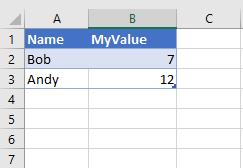
Figure 1. Example table layout
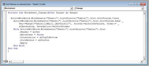
Figure 2. Code module
2019-05-28 17:37:49
Brian Smith
If I have two columns, one column (A) with a list of names, and then the second column (B) with a list of numbers, and I want this macro to sort based on the data entered in B, how would I modify the macro so that column A moves with it? So, if I have two names, Andy and Bob in A1 and A2, then I put 12 and 7 in B1 and B2, so then the macro automatically sorts it so that 7 is on top of 12, how would I make it so that Bob (value of 7) moves to the top (above Andy, value of 12)?
2017-12-04 10:34:35
Peter Atherton
Sidney Mashiloane
Create a helper column, say In column C. In C3 enter the formula =(B3-$A$1)+1/COUNTIF($B$3:$B3,$B$3:B3) and copy down. You can now sort the list on column C. If you open the developers tab you can record the macro and edit the range for next time it is run.
Personally I prefer to leave the original data as entered - you can use formulas to show the last 10 values or so. To get the date type:
=INDEX($B$3:$B$103,MATCH(SMALL($C$3:$C$103,ROWS($1:1)),$C$3:C$103)) and copy down as many items you want.
to get the items type:
=INDEX($B$3:$B$103,MATCH(SMALL($C$3:$C$103,ROWS($1:1)),$C$3:C$103))
{fig}
(see Figure 1 below)
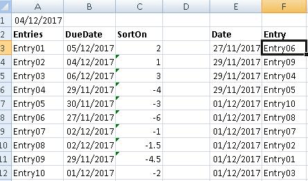
Figure 1. Index
2017-11-27 08:28:38
Sidney Mashiloane
Hi Allen, thanks a million for the codes given above, they almost answer my question. My question: in cell A1 i enter Today(), which returns today's date. in column A from A2 downwards i have entries and in column B i have due dates. i want excel to sort the rows using the dates in column B by using the dates displayed in cell A1 i.e. all the items with the date equal to or closer to A1 should move up and those still far should move downward. can you help with that please
thanking you in advance
cheers
2017-11-15 11:13:52
Willy Vanhaelen
@Chloe
You probably had already a row numbered 1. If you enter 1 again in a new row it joins the other number 1 after sorting and you have then 2 rows numbered 1.
2017-11-13 15:34:07
Chloe
Hi!
Say I also wanted the row numbers to auto-adjust, how could I go about doing that?
What I mean is, when I enter say 1 in row 20, I want row 20 to go to the top and all the other numbers to follow suit. Right now, I'm ending up with two rows numbered 1.
Thanks
2017-11-13 10:24:56
Chloe
Hi!
Say I also wanted the row numbers to auto-adjust, how could I go about doing that?
What I mean is, when I enter say 1 in row 20, I want row 20 to go to the top and all the other numbers to follow suit. Right now, I'm ending up with two rows numbered 1.
Thanks
2017-11-10 05:56:11
Willy Vanhaelen
@Ken Varley
Look at my post of 2013-11-17. With that technique you can start entering in any column and when the row is sorted the cell pointer follows the sorted row and you can immediatly continue in other columns.
2017-11-09 04:59:29
Ken Varley
Another way would be to sort the data on the last item entered. Say the data was in columns A to E, then the sort would take place after completing E
From Above " If Not Intersect(Target, Range("A:A")) Is Nothing Then"
Alter to " If Not Intersect(Target, Range("E:E")) Is Nothing Then"
-------------------------------------------------------------------------------------------
Another alternative might be to create an Input area (row 1), and sort the data only when all of the cells in the input area contain a value. (Resetting the input area to blanks afterwards)
2017-10-28 05:56:54
Willy Vanhaelen
@Adrian Allen
The Worksheet_Change event is only triggered if the content (formula) in a cell in that worksheet changes. It isn't triggered if only the result of that formula changes. So what you are trying to do can't work :-(
2017-10-27 14:40:07
Adrian Allen
Hi,
Is there a way to do this when the data say in column A is taken from a different worksheet within a workbook using the reference formula
So basically data in sheet1 is put into a tablet in sheet2 if it meets certain criteria, so the data isn’t manually input into the column which requires auto sorting
Any ideas?
2017-04-27 04:16:48
Bob
Additional info: Row 8, Row 20, Column A and Column AD are all blank.
Thanks again!
2017-04-27 04:04:29
Bob
Hi there, amazing post, thank you for sharing VBA wisdom! Already subscribed :)
I was able to adapt the basic code from the original post so it works but I'd like to use the code from the 17 November 2013 post so the entry doesn't disappear. Please write the code for the following:
Table goes from B9 to AC19 with every 2 columns merged. So B-C is the first column, D-E the second, all the way to AB-AC for a total of 14 columns. Row 9 is header, with rows 10-19 containing the data. I'd like all the data to be sorted by column L-M, and all columns on either side to follow sorting (B-C to AB-AC). And of course entry stays with the right row.
Thanks in advance for your help!
2017-03-25 03:08:31
Allen
Johan
From your note, you split the values in column 1(A) into numbers and letters, and put them in column 2 (B) and column 3(C) respectively. You note you do this with code, so I assume you are familiar with VBA and macros. After you split the values into separate columns, you want to sort on column 2 ascending, then column 3 ascending - this is a cascading sort, where the order is important. Here is a simple macro:
#############
Sub SortBC()
With Range("A1", Range("E" & Rows.Count).End(xlUp))
.Sort Key1:=.Columns(2), Order1:=xlAscending, _
Key2:=.Columns(3), Order2:=xlAscending, Header:=xlGuess
End With
End Sub
#############
This would be placed after you split the values into columns b and c. You'll need to adjust the range. You can add more keys as you need.
2017-03-24 06:38:41
Johan
Hi There,
VBA Excel Programming problem!
I had an Add Button on a form. When Clicked, two txtBoxes and a listBox values are written onto a spreadsheet into Column A ("Numbers"), Column D("Size") and Column E("Time") as AM/PM.
Column A gets any sort off numbers like 1,2,6,7B,7A, 21,22,23, 18B,18C,18A, ......33,35,27A,27B, till last number.
Then I split,"with a splittext coding in a Module" the values in column A to Column B(only Numbers) and Column C(only letters) which I hide from the client.
The Problem:-
Now I want to Automatically after CLICKING the ADD BUTTON, sort Column B(Numbers) in ascending order from small to large and Column C(Letters) to follow in ascending order but to KEEP IT'S position or place with there corresponding Number.
And then Lastly to sort Column A, Column D and Column E using the info from columns B:C
The Data in Column A , D and E will be used else where in the program for the customer to see on a Form but in an ASCENDING Order!!
I have had looked to most Forums for this solution but yet to find my degree of problem solving.
Hope someone is able to assist me.
Thx in advance.
2016-10-04 03:44:19
sidney
hi
my request is a little different. i want the rows to automatically move up in descending order depending on the date entered in column A on each row. This means today's dates will be topmost, followed by tomorrow and so on. Past dates will remain at the top also, above today's date. can you please help
thanking you in advance
2016-09-17 22:03:45
sherlyn
hi, i have a data on column A.
(ex. )
I. A steel bars
a.1 50mm x 25mm x 600mm
a.2 30mm x 25mm x 600mm
a.3 60mm x 25mm x 600mm
B flat sheets
b.1 25mm x 50mm x 800mm
b.2 35mm x 50mm x 800mm
b.3 40mm x 50mm x 800mm
if i will delete the a. 1 , a. 2 will automatically became a. 1, as a. 3 became a. 2. or if i will delete the entire A the entire B will automatically became A. how would i suppose to do that? is it possible?
tnx a lot!!!
2016-08-04 11:46:56
Willy Vanhaelen
@Alex
The solution I proposed in my comment of 17 November 2013 solves your problem.
This macro sorts by column A. As soon as you make an entry in that column the record is sorted but the cell pointer follows instantly and jumps to the new position of the record so you can smoothly continue entering data in the other columns without any interruption.
IMPORTANT: the macro must be entered in de code page of the sheet containing your table. Simply right click the sheet's tab and select "View code". That's the place to be.
2016-08-04 06:27:27
@Alex
You need to decide what event is going to trigger the sorting, if you are unhappy with the solutions that Willy VanHaelen has proposed (which sort immediately upon entry of the cell that triggers the sorting).
Unfortunately, Excel cannot predict whether or not you are going enter the data into cells I-N, so it looks like you'll have to press a button to tell it.
You might consider, given that you are entering up to 14 pieces of data per entry, using a UserForm this can give you a more user-friendly interface, and to apply a more rigorous data validation checks before accepting input.
2016-08-03 14:45:48
alex
hi there, i've been trying and trying but to no avail to figure out this macro.
i have a document with columns A-N with headers.
I need it to sort by Column A but not until i have finished entering everything after that. i sometimes wont fill in I-N till a little later but sometimes i will.
Any way to do this? PLEASE PLEASE HELP
2016-08-01 22:33:48
robert
how can i use these macros? what will i type?
2016-07-06 13:46:42
Willy Vanhaelen
@Pramodkumar
This can only be realised if your data table is the entire columns F to W, has headers and columns E and X are entirely empty. Then this macro can do the job:
Private Sub Worksheet_Change(ByVal Target As Range)
If Target.Column <> 7 Or Target.Columns.Count > 1 Then Exit Sub
Dim tmp As Variant
tmp = Cells(Target.Row, 8).Formula 'save contents
On Error GoTo Enable_Events
Application.EnableEvents = False
Cells(Target.Row, 8) = "#"
Range("F1").Sort Order1:=xlAscending, Key1:=Range("F1"), Key2:=Range("G1"), Header:=xlYes
Cells(Application.Match("#", Columns(8), 0), Selection.Column).Select
Cells(Selection.Row, 8) = tmp 'restore contents
Enable_Events:
Application.EnableEvents = True
End Sub
The macro has also the advantage that the cellpointer follows the record to it's new position after the sort.
2016-07-06 03:13:35
Pramodkumar
I have datas in sheet1 ranging.F10:W28 The column(F10:F28) reffesrs to date and column(G10:28)for bill Numbers. Can I have a single vba to sort dates first and then the bill nos?
Ie.In case of same dates, sort data based on bill Nos
Thanks a a lot
2016-06-14 11:09:22
Michelle
RE: Auto Sorting Linked Sheets:
Master data sheet (sht) has 7 other shts linked to it. Each sht displays that section's related data from the Master sht.
Need to auto sort only the linked shts by last name, then first name (which I thought should have been easy), but still need to keep all associated line data.
I have done conditional format for blank rows to be "zz" and used white font to hide. The data formulas linking to the master sht go to 301 lines, so potential of a lot of blank lines in-between rows of data. I have worked out all my formulas and links to each sections' sht, but having issue getting the auto sort working and what mechanism to use to trigger auto sort within the linked sheets (not using name since it is first data cells keyed, would like to use Section ID). I have been reading your message board, which has a wealth of information, but I have not been successful in getting auto sort working.
**Using Excel 2013 version.
Master Sht: only 7 key-able fields (columns), rest are all formulas (13 columns).
Linked Sht: only 13 columns of data displayed/linked from Master Sht.
(Project: Employee Yrs of Service Awards/Recognition. Spreadsheet for determining when employee is eligible for Yrs of Svc award broken down by each section.)
Your assistance and patience is very much appreciated. TY.. M
2016-05-22 09:38:03
I am new at code and need help on automatically sorting from [row 20 down to row 590, columns A:L] by dates (older to newer) that i enter in column A20:A590 after entering whatever data i choose to enter in that row.
Note: rows 1 through 20 must remain unaltered.
Can someone please help me.
2016-04-30 02:53:24
Kashish Shah
You are God. Thank you so much for helping.
2016-04-03 07:04:51
nnd
i have spreadsheet which contain type of product for which different cost is to be mentioned i have prepared to columns with product and cost now i want to pick up the cost for product when i enter the product name
2016-03-02 10:29:34
I see two approaches described here.
1. Use VBA with an appropriate event-driven trigger. Fine. Not for those that don't enjoy VBA.
2. Use the function Large(). Also fine, but it only works if the data is only a single field.
There is another way using
Rank() (applied to the input data)
Match() (just once, looking for the nth rank)
and
Index() (once for each desired field from the database)
This works fast, is efficient, works for any number of fields with the data in columns or rows.
Easy enough. Details left to the reader.
2015-08-21 12:40:49
Willy Vanhaelen
@Katie
With some adjustments, the macro I posted 17 November 2013 will do the job:
Private Sub Worksheet_Change(ByVal Target As Range)
If Target.Column <> 2 Or Target.Columns.Count > 1 Then Exit Sub
Dim tmp As Variant
tmp = Cells(Target.Row, 1).Formula 'save contents
On Error GoTo Enable_Events
Application.EnableEvents = False
Cells(Target.Row, 1) = "#"
Range("A5").Sort Key1:=Range("B5"), Order1:=xlAscending, Header:=xlNo
Cells(Application.Match("#", Columns(1), 0), 2).Select
Cells(Selection.Row, 1) = tmp 'restore contents
Enable_Events:
Application.EnableEvents = True
End Sub
For the macro to work correctly cells A4, B4 and column C must be blank.
The macro has also the advantage that the cellpointer follows the record to it's new position after the sort.
2015-08-19 08:03:13
Katie
Hi,
I need someone to write out the code for me please! basically for colum B from 5 so (B5) to around B50 I want that colum to be decending so the oldest date first (the dates are people birthdays and I need the oldest person at the top) and also there names before them in colum A from A5 to move with them. And this sheet to automatically move them when a new name and d.o.b is added!
Please could someone help ive tried changing other peoples posted codes and I just cant get it to work :/ thanks in advanced!
2015-07-30 11:18:50
Amber
I would like to automatically sort by date in column G and the information next to it on both sides to stay with it. I would also only like to sort a portion. For instance I would like to sort G2-G54 by date and then be able to sort G56-G87 the same way. I do not want to lose the data to the left and right of column G. I want it to move with column G based on the sort location.
2015-05-31 12:35:22
Ryan Margerison
Hello there I have an excel workbook which is a football league table system, I want it so that every new result input auto sorts the new league table based on the results and the league table has combined if statements to count the wins and I have formulas for calculating points etc. I just need to sort it out so that the table auto sorts in one sheet based on new results in the other? Can anybody help me with this?
2015-05-04 23:38:37
Dani
Hi i just started using macro and i'm hoping to sort my data by color this is the command i'm using but it doesn't seen to be working can somebody guide me as to what i'm doing wrong
Private Sub Worksheet_Change(ByVal Target As Range)
ActiveWorkbook.Worksheets("Plans").Sort.SortFields.Add(Range("M3:M1125"), _
xlSortOnCellColor, xlAscending, , xlSortNormal).SortOnValue.Color = RGB(253, _
233, 21)
ActiveWorkbook.Worksheets("Plans").Sort.SortFields.Add(Range("M3:M1125"), _
xlSortOnCellColor, xlAscending, , xlSortNormal).SortOnValue.Color = RGB(242, _
220, 219)
ActiveWorkbook.Worksheets("Plans").Sort.SortFields.Add(Range("M3:M1125"), _
xlSortOnCellColor, xlAscending, , xlSortNormal).SortOnValue.Color = RGB(228, _
223, 236)
ActiveWorkbook.Worksheets("Plans").Sort.SortFields.Add(Range("M3:M1125"), _
xlSortOnCellColor, xlAscending, , xlSortNormal).SortOnValue.Color = RGB(197, _
217, 241)
ActiveWorkbook.Worksheets("Plans").Sort.SortFields.Add(Range("M3:M1125"), _
xlSortOnCellColor, xlAscending, , xlSortNormal).SortOnValue.Color = RGB(217, _
217, 217)
With ActiveWorkbook.Worksheets("Plans").Sort
.SetRange Range("M3:M1125")
.Header = xlYes
.MatchCase = False
.Orientation = xlTopToBottom
.SortMethod = xlPinYin
.Apply
End With
End Sub
2015-04-26 11:40:36
Yaw Asante
please show me how I can enter sudent ID number in a cell and return the nane that bears the name of the ID to bring student exams record from a stdent sammary exam record. thank.
2015-03-31 03:14:53
Babulal Gandhi
Hi Friends
I Have Phone Numbers Like This To Sort By Rows
66-66970877, 22-34567, 8764576890, 333-7465 (Column A1,Column B1,Column C1,Column D1)
These Are Phone Numbers Which I Have To Short For Small To Large Or Large To Small
Sorting Data In Row P1 To S1
22-34567, 333-7465, 66-66970877, 8764576890 (Column P1,Column Q1,Column R1,Column S1)
Column P1 = small($a1:$d1,1)
Column Q1 = small($a1:$d1,2)
Column R1 = small($a1:$d1,3)
Column S1 = small($a1:$d1,4)
These Formula Works Great On Without (-) Numbers.
I Need Formula To Ignore (-)
Numbers Before (-) Is Area Codes. If I Remove (-) With Find & Replace. I Will Get Confuse In Future As I Can't Differentiate Area Code And Phone Number.
If There Is Solution In Macro
I Want To Short Telephone Numbers In Three Rows After Mobile Numbers In Other Three Rows.
P1-Telephone Number, Q1-Telephone Number, R1-Telephone Number, S1-Mobile Number, T1-Mobile Number, U1-Mobile Number
I Need A Macro
1. Ignores The (-) Value In All Phone Numbers
2. Check First Digit Of Phone Numbers.
3. If First Digit Start's With Nine(9). If There Is Any Single Phone Number In A1, B1, C1, D1 Starting With Nine(9)(It's Mobile Number) Put Into S1. Else If There's Two Numbers Starting With Nine (9) Place It In Row S1 And T1 In Ascending Or Descending Order
4. If First Digit Start's With Eight (8). If There Is Any Single Phone Number In A1, B1, C1, D1 Starting With Eight (8) Put Into Q1. Else If There's Two Numbers Starting With Eight (8) Place It In Row Q1 And R1 In Ascending Or Descending Order
Like Wise For Other Digits Too
Thanks & Regards
Babulal Gandhi
2015-03-05 19:03:21
Kenneth
#1 Salads 1234
Barrens, Alicia 2222
jackson, Peewee 1515
Johnson, Aaron 4242
Pooty, Tang 3456
Shields, Derick 7689
Shields, Ruby 9870
Spencer, Kenneth 9999
Zebra 6767
Obama, Barack 1111
Andersson, Paul 1236
This is sample data. I want to be able to automatically resort the data alpabetcally when new data is added. If I add a new Name and ID I want to resort automatically. There is no column heading and I AM A NOVICE, a complete NOVICE to VisualBasic. Can someone help me pleaseeeee??? Thanks in advance, Ken
2015-03-01 07:36:50
OptimusPrime
@Micro
If you want the values of result in column C of Step 7 to be sorted
do the following:
Step 8: Write S.NO. in cell E1
Step 9: Write numbers from 1 to 9 in cell E2 to E10
Step 10: Write SORTED NON-DUPLICATES in cell F1
Step 11: Write =IFERROR(LARGE($C$2:$C$9,E2),"") in cell F2 and drag it to F9
observe values in Column F
2015-03-01 07:19:57
OptimusPrime
@Micro
Follow the instructions :
Step1: Write HELPER in cell A1
Step2: Write 1 in cell A2
Step3: Write VALUES in cell B1
Step4: Write all desired values including duplicate values in cells from B2 to B10
Step5: Write NON-DUPLICATES in cell C1
Step6: Write =IF(COUNTIF($B$2:B3,B3)=1,A2+1,A2) in cell A3 and drag it till A10
Step7: Write =IFERROR(VLOOKUP(ROW()-1,$A$2:$B$12,2,FALSE),"") in cell C2 and drag it till C10
Observe values in Column C
revert back if any problem exists.
2015-02-28 07:41:40
Miro
@ Willy Vanhaelen
I dont think this is what i wanted. I want actual data to be sorted out and non duplicates to be listed in that other sheet. As bellow example :
A B C
1 348 27.80 351
2 348 27.80 351
3 351 27.80 348
4 351 27.80 342
5 351 27.80 342
6 348 27.80 342
Values in column A and C are repeating them self's , i need formula to get each of ( unique ) value in some third column ( or sheet ) so result should be :
D
351
348
342
We manage to solve this with below formula , another problem a rise i cannot adjust formula to take both columns ( A & D ) when checking , only works when one column is in question .
Thank you everyone for help.
=IFERROR(INDEX(N$4:N$136,MATCH(0,INDEX(COUNTIF($B$3:$B5,$N$4:$N$136), 0))),"")
2015-02-27 06:15:24
Willy Vanhaelen
@Rhys W
- Select the cell you want to delete and press [Ctrl]+[-] (minus key).
- In the Delete dialog that pops up, check 'Shift cell up' and click [OK].
@Miro
- Copy your data in column A to column D.
- With you data still highlighted in column D click 'Remove Duplicates' in the 'Data Tools' section in the Data tab of the ribbon and click OK.
2015-02-26 10:20:57
Miro
I need help with this one. I have one column lets say A1 : A38 that have some values / text . Those values can repeat themselves through A1 : A38 many times . I would like to get in another row or even sheet only one of each of those values or records.
For Example : A1 have TB231 ; A2 TB236 ; A3 TB555 ; A4 TB555 ; A5 TB231 etc , now in separate sheet or row i should get only one of those , it dosent matter how much it has same records i just need that i get value of all different in separate sheet or row.
Results of example should be : D1 TB231 ; D2 TB236 ; D3 TB555 , i tried with IF function but for 38 or more rows would be huge so maybe there is other easier way.
2015-02-26 09:57:57
Rhys W
I'm using this code to automatically sort two columns in a-z order as I enter new Names, however, how do I make it so that when I delete a Name, the rest of the data under it moves up and takes its place?
2015-02-24 14:13:48
Willy Vanhaelen
@Celia F.
Well simply write what you want to do:
The basic command is: Range("A1").Sort
Then you have to add a key to sort by: Key1:=Range("C1")
Now add the sort order: Order1:=xlAscending
Tell Excel if there is a header: Header:=xlYes
If you want a second key to sort by: Key2:=Range("A1")
If you want a different sort order for this one, simply add it: Order2:=xlDescending
Now bring this all together separated by comma's (no comma after Sort):
Range("A1").Sort Key1:=Range("C1"), Order1:=xlAscending, Header:=xlYes, Key2:=Range("A1)
That's it.
2015-02-23 14:30:27
Celia F.
How do I do a macro for auto sort for multiple columns? I want it to sort column C then column A.
2015-02-14 12:59:25
Chris
Willy,
Thanks! I had to do some playing around with the ranges since I have a lot of data spread throughout the page, but it worked perfectly. Thanks again!
2015-02-14 06:00:29
Willy Vanhaelen
@ Chris
Try this:
Range("A:B").Sort Key1:=Range("B1"), Order1:=xlAscending, Header:=xlYes
2015-02-14 05:23:18
Pascal
Hi guys I want to create a contact list.
First Column will be Company/Organisation Name, the second column will be Department and the third column will be the Name. The rest columns will be theirs telephone numbers, fax numbers, emails addresses etc.
I just want the first 3 columns to be connected together in alphabetical order.
I tried with the Data and Sorting but nothing!!!!
2015-02-13 13:53:23
Chris
This works great for what I'm trying to do except for one little issue. Say I have a 3 column worksheet but I only want the first 2 columns sorted by the data in column B, and want column C to remain constant? I'm new to using macros so be gentle. Thanks
2015-02-13 11:54:16
OptimusPrime
Hi Sireen,
If you have MSoffice 2007 or 2010, then check this out:
Home Styles Conditional Formatting New Rules
Hope you may find a solution for yourself.
By the way, how the data is automatically changing in cell, are you taking from outside Excel or from other excel sheet ?
Regards.
2015-02-12 05:57:27
Sireen
Hi,
I need for excel to automatic change the data in one column to different wording into another column.. as the first one is generated form a software that we use, but the analysis should be stated in different wording .. like the key to a map .. every green colour represent forest !!
Is it possible ?
Thanks,
Sireen
2015-02-02 23:25:47
OptimusPrime
Hi Tushar,
Check this out. You may find a solution for your query.
https://www.sendspace.com/file/p4dn9o
Regards.
2015-02-02 23:21:24
OptimusPrime
Sorry Guys, there was a mistake in my previous post.
The correct one is as follows:
Step1: Enter serial no 1 to 10 in cells A1 to A10 (S.No.).
Step2: Enter any values in cells B1 to B10 (Item Qty.).
Step3: Enter any object names in cells C1 to C10 (Item Name).
Step4: Enter formula =RANK(B1,B$1:B$10)+COUNTIF(B$1:B1,"="&B1)-1 in cell D1. Drag till D10. (Item position)
Step5: Enter formula =C1 in E1 and drag till E10. (Item Name as is)
Step6: Enter formula =LARGE($B$1:$B$10,A1) in F1 and drag till F10. (Desired Item qty. in order)
Step7: Enter formula =IFERROR(VLOOKUP(A1,D$1:E$10,2,FALSE), VLOOKUP(A1,D$1:E$10,2,TRUE)) in cell G1 and drag till G10. (Desired Item Name in order).
Watch carefully, Your Desired Item qty. and item name would be in Cell F1 to G10.
2015-01-31 00:42:41
Tushar
Hi,I have to maintain student weekly attendance form.
My excel sheet having 6 sheet name
mon,tue,wed,thu,fri,final,new
from mon to fri i have students name with enrollment no, and attendance.
in final sheet i have student list who havent appear three consecutive days
0 means present
1 means Absent in final sheet column m
i want only those students enrollment no , name in new sheet who having value 1 in final sheet column m please help
2015-01-27 17:51:08
OptimusPrime
Guys,
Check this out for a better solution and Do as i write:
Step1: Enter serial no 1 to 10 in cells A1 to A10 (S.No.).
Step2: Enter any values in cells B1 to B10 (Item Qty.).
Step3: Enter any object names in cells C1 to C10 (Item Name).
Step4: Enter formula =RANK(B4,B$4:B$16)+COUNTIF(B$4:B4,"="&B4)-1 in cell D1. Drag till D10. (Item position)
Step5: Enter formula =C4 in E1 and drag till E10. (Item Name as is)
Step6: Enter formula =LARGE($B$4:$B$16,A4) in F1 and drag till F10. (Desired Item qty. in order)
Step7: Enter formula =IFERROR(VLOOKUP(A4,D$4:E$16,2,FALSE), VLOOKUP(A4,D$4:E$16,2,TRUE)) in cell G1 and drag till G10. (Desired Item Name in order).
Watch carefully, Your Desired Item qty. and item name would be in Cell F1 to G10.
If still got problem, download the excel sheet, its protected and the password is password. change value in current cell and press Enter. Watch the last two columns.
https://www.sendspace.com/file/5g6uqg
Still in problems ? let me know.
2015-01-21 09:27:46
Chris
Hi, I'm trying to automatically resort a constantly changing block of data (A80:P179) by the J column, descending by value. My data does not have headers.
Could you please help me out with this and show me where I would adjust the ranges for different data?
Thanks you in advance,
Chris
2015-01-15 12:06:31
Brenda
Is there anyway I can alphabetize a list of names automatically and also transfer their specific information at the same time with one formula.
2015-01-15 12:04:20
Brenda
Is there any way I can add new names to be sorted in alphabetical order and still have their pertinent data changed automaticall along with them when I add a new person to the list? I am very new at this process
2015-01-09 09:47:47
Glenn Case
Mickale:
You can either record a macro of the sort you want, or use the examples in the tip and comments in order to produce a macro which does the basic sort. This macro would be located in a code Module. You can then use an event macro as per the tip to test whether a change to the worksheet was in the range of interest (hours), and if so, call the first macro.
2015-01-08 13:32:12
Mickale
I am new to macro codes and I really need some help! I am trying to write a code for my worksheet that will automatically sort "total hours" from least to greatest. My first column has names and then I have their total number of hours worked in the next column. I have headers in the worksheet and it needs to change everytime the hours worked is changed.
Any help would be greatly appreciated! Thanks
2014-12-24 05:21:24
Barry
@Julie Meng
I would use a Case select to filter out the worksheets either that I want the sorting to occur on or as an exclusion list depending if you'll be adding extra sheets to the workbook that either need to be auto-sorted or not. The code below works on an exclusion list
Private Sub Workbook_SheetChange(ByVal Sh As Object, ByVal Target As Range)
On Error Resume Next
Select Case Activesheet.Name
Case "List", "Main", "X", "Y", "Z"
CaseElse
If Not Intersect(Target, Range("H:H")) Is Nothing Then
Range("B12").Sort Key1:=Range("B13"), _
Order1:=xlDescending, Header:=xlYes, _
OrderCustom:=1, MatchCase:=False, _
Orientation:=xlTopToBottom
End If
End Select
End Sub
2014-12-23 15:41:26
Julie Meng
Hello Everyone,
I am using this for my entire workbook. I would like to keep this from running in my first 5 worksheets. This is what I am running right now:
Private Sub Workbook_SheetChange(ByVal Sh As Object, ByVal Target As Range)
On Error Resume Next
If Not Intersect(Target, Range("H:H")) Is Nothing Then
Range("B12").Sort Key1:=Range("B13"), _
Order1:=xlDescending, Header:=xlYes, _
OrderCustom:=1, MatchCase:=False, _
Orientation:=xlTopToBottom
End If
End Sub
I am Auto sorting column B when a change is made to column H.
Please let me know how I can keep it from running on my worksheets named List, Main, X, Y and Z.
I have several worksheets and need this auto sorting for all of my sheets but the first five. There is no way in hell i'm setting this up in each individual sheet, way to much work.
Thanks for this Allan, it is making my work so much easier!
Hope I can get this figured out before I pull all my hair out!
2014-12-03 19:03:37
Amanda
Hi there. I am creating a spreadsheet that pulls data from several other worksheets. I am trying to get it to sort automatically by data in column L rows 4-18, header is in row 3. I have tried several different macros, but it keeps disconnecting my data from the rest of the columns. all data that needs to be sorted is in A3:AB18. Help!
2014-11-05 09:22:12
@ Bill
Check the code below. Here are the assumptions
- you will be entering date in only B & C.
- you will enter B then C.
If you expect to sort after entering in a specific column and you are entering more than just B & C (e.g. you are entering in A, B, C, D, and E) and you want to sort after entering in E, then change the Intersect to look in column E.
Private Sub Worksheet_Change(ByVal Target As Range)
On Error Resume Next
If Not Intersect(Target, Range("C:C")) Is Nothing Then
With ActiveSheet.Sort
.SortFields.Clear
.SortFields.Add Key:=Range("B:B"), SortOn:=xlSortOnValues, Order:=xlAscending, _
DataOption:=xlSortNormal
.SortFields.Add Key:=Range("C:C"), SortOn:=xlSortOnValues, Order:=xlAscending, _
DataOption:=xlSortNormal
.Header = xlYes
.MatchCase = False
.Orientation = xlTopToBottom
.SortMethod = xlPinYin
.SetRange Range("B2:C" & CStr(ActiveSheet.Rows.Count))
.Apply
End With
End If
End Sub
For a more complex problem, say you want to sort after A through E on a row are complete then you would wrap an If statement around the With'''end With. The "If", in this case is whether all input is complete for the row. Below is the code for this...
Private Sub Worksheet_Change(ByVal Target As Range)
On Error Resume Next
If Not Intersect(Target, Range("A:E")) Is Nothing Then
If RangeInputComplete(Range("A" & Target.Row & ":E" & Target.Row)) Then
With ActiveSheet.Sort
.SortFields.Clear
.SortFields.Add Key:=Range("B:B"), SortOn:=xlSortOnValues, Order:=xlAscending, _
DataOption:=xlSortNormal
.SortFields.Add Key:=Range("C:C"), SortOn:=xlSortOnValues, Order:=xlAscending, _
DataOption:=xlSortNormal
.Header = xlYes
.MatchCase = False
.Orientation = xlTopToBottom
.SortMethod = xlPinYin
.SetRange Range("A2:E" & CStr(ActiveSheet.Rows.Count))
.Apply
End With
End If
End If
End Sub
Public Function RangeInputComplete(rng As Range)
Dim cel As Range
RangeInputComplete = True
For Each cel In rng.Cells
If Len(cel.Value) = 0 Then
RangeInputComplete = False
Exit For
End If
Next cel
End Function
2014-11-04 17:12:47
Bill
The original macro works great, but I want to now sort by 2 columns, "b" then "C". What do I add to the macro to accomplish this?
Thaks
2014-10-28 15:37:59
@ Samuel
First, this is probably something that would best be covered by sending an email to Allen's Help Wanted email . It's listed at the bottom of every week's Tips newsletter. If you aren't already a subscriber, I strongly suggest you do. It's part of my on-going education and he doesn't pass on your information to others who are going to send you a bunch of junk mail.
The advantage of submitting that way would be several people will provide their methods for solving each problem and you are more likely to get an answer that fits your needs. The URL is http://excelribbon.tips.net/contact.html?awt_l=EQOC_&awt_m=JcuXuyTnu4R74X
OK...all of that aside I am going to give two approaches you might use. I am starting with the assumption that your Master List has each student by name plus their cumulative score. For the sake of this I will also assume those are columns A and B, respectively, and the names are sorted in alphabetical order.
One approach would be to sort A:B by B, descending then populating another column (let's say it's column C) with the ranking.
Assuming you start in row 2, then the formula for C2 would be (without the quotes) "=If(B1=B2, C1,Row()-1)"
The B1=B2 test's for ties and both would get the same ranking. Otherwise their ranking would be the Row number with an adjustment for the row where the data starts.
Once done, copy-pastespecial/values then you can re-sort on the names.
The second approach would be to read the the data into an array with a two-field data type: Name & Grade. DIM arr(1 - NumberOfStudents).
Load the data from Master into the array, then sort the array on Grade, descending.
When reading from the array, for each entry into the array FIND the ROW with the name and plug the current i of the array. Roughly, the code looks like this.
For i = Lbound(arr) to Ubound(arr)
RowNum = Application.WorksheetFunction...Row
ws.cells(RowNum,RankingColNum) = i
Next i
The last thing that I can think of that you might want to do is put the class ranking back on the report card sheets. Assuming you have the student's name on that sheet the a vlookup(StudentName, Master!A:C, 3, False) will return the Class Ranking.
Like I said, if you would like the input of several people, send the message to Allen. Hope this helps.
2014-10-27 07:04:34
please I need help. I have just developed a VBA app. in excel that automatically process report card for a class in a school. now I want to be a bale to assign class position to each pupil in class automatically. each pupils result is on a different sheet. I have a master sheet that collects the total scored for each pupil.
2014-09-09 03:19:55
Michele
Hi
I would really appreciate it if someone could help me with my query.
I have a table with data inserted through Vlookup formula. I want a specific column (C) to be automatically sorted in descending order depending on its value. Can you please help me with the VBA formula I need to input? I have attached the table below FYI.
The data including the heading runs from B9 to K24.
Basically I want to sort the table depending on the values of C10 to C24 in a descending order.
Component Ingredients Product Code Weight Kg/L % Allergen, if present
Roast beef 35 0.100 28.33% nil 0 0 0 0 0
Rock melon #N/A 0.070 19.83% #N/A #N/A #N/A #N/A #N/A #N/A
Whole grain mustard #N/A 0.040 11.33% #N/A #N/A #N/A #N/A #N/A #N/A
Melon #N/A 0.070 19.83% #N/A #N/A #N/A #N/A #N/A #N/A
Tomato Wedge #N/A 0.026 7.37% #N/A #N/A #N/A #N/A #N/A #N/A
Parmesan #N/A 0.020 5.67% #N/A #N/A #N/A #N/A #N/A #N/A
Pesto 5 0.010 2.83% nil 0 0 0 0 0
Diced tomato #N/A 0.005 1.42% #N/A #N/A #N/A #N/A #N/A #N/A
Arugula #N/A 0.005 1.42%
Sundried tomato #N/A 0.004 1.13%
Lolorosso #N/A 0.002 0.57%
Kalamata olive #N/A 0.001 0.28%
Chive #N/A 0.001 0.28%
Wheat bread 400206 1 slice #VALUE!
0 #N/A 0.000 0.00%
2014-08-21 17:03:09
Lost Boy
Hello,
I want this but for rows. I need a code that will auto sort my row of totals (which are the end of a chain of formulas – the total cells themselves included)so that cell B12 is always the highest number and cell O12 is always the lowest number. While keeping the data in the columns above in tact with the number in row 12 as they are the data that sums to the totals in that row. My totals sheet uses column A for date ranges (starting at A3 and going to A12) and columns B through O are states (all on row 2). There are sheets for each state that connects to the totals page and provides the data for all the cells. How can I make it auto sort so the state with the highest number (which is the sum of - for example B3-B11)is always on the left and the lost number always on the right? Let me know if you need any more information. Thank you.
2014-08-07 04:49:32
Colin
Is there anyway of automatically updating without the need to input anything. I have a table that receives updates automatically from a server, but I need it to auto sort every 2 seconds.
Thanks in advance
2014-07-30 07:11:54
Salik Khatri
Hi!
Your thread is really helpful, exactly what im looking for!!! However im kinda new to this deep dark world of excel (ofcourse, i know the basics) bur recently my company has had an increased level of activity which has left me no choice but to explore new techniques to sort out data efficiently and on hand at all times.
The idea is simple, i've made a list of invoices which need to be paid. Colums include supplier, description, amounts in AED & USD, date, due date etc..the usual sutff. I calculate the number of days due by subtracting the due date with today's date [i use =today ()] to do this. Now that i have the number of days, i want to sort the entire row in an ascending order (i.e. overdue or past due - reflected as a negative figure).
The colums start with A: Suppliers and run through to I: Due in(Days)
Many thanks!
Salik Khatri
2014-07-18 15:35:03
Rocky
Hi,
I have two questions:
1. If i have values in rows 1-9 and Im typing in a value in row 20. As it is today row number 20 wont count until row 1-19 are complete. What do I need to do to get every row in colum A count all the time?
2.If I have ex row number 5 as a parent and row number 6 is a child by using this group function. As Im entering a value for parent I want the child to move around with parent. Is this posible to do?
2014-06-18 15:21:57
DRB
I like it, but with both excel and world cup fever, I have a harder issue.
I have a list of games/times/teams and scores (and calculate points and goal difference). Below that I have equations that sum the points and goal differences for each world cup group. I want to sort these cells that contain equations every time I enter a score above (so I know the top two teams in each group). Is there any way to sort those?
DRB
2014-06-07 23:11:42
minhruj
Anyone help me in this issue, please?
Within one sheet I have 8 databases (all no heading), which can be listed as K8:Q11, K12:Q15,... What I need is an automatic procedure to sort these databases' rows separately . The procedure must comply with 2 levels: First, sort by column Q, order largest to smallest, then sort by column P with the same order (data in these 2 columns are all numeric format.
Thanks so much!
2014-05-28 03:19:44
rashmi
i want to add a fixed date, say 30-apr-2014 everytime I run my macro how do i do this? please could you help
2014-05-20 05:12:29
is it possible to please send me a template which i can use
2014-03-29 11:39:17
nitin
Hi!
Got the solution.
But 2 queries:
1. What does Key1:=Range("A2") refer to?
2. The regional settings on my laptop are Indian but the date format (which was earlier accepting indian format of input viz. dd-mmm-yyyy) is now accepting only american format - ie: mm-dd-yyyy but is displaying in dd-mmm-yyyy format.
eg.: if i enter "2-1" the date automatically converts to "01-feb-2014"
& if i enter "23-5" it converts to "23-05-2014" but if i enter "5-23" it converts to "23-Jan-2023"
Can you please guide to resolve this?
BTW, I forgot to mention that the sorting is done on the date column
the macro i use is:
Private Sub Worksheet_SelectionChange(ByVal Target As Range)
On Error Resume Next
If Not Intersect(Target, Range("d17:d1000")) Is Nothing Then
Range("d17:i1000").Sort Key1:=Range("d1"), _
Order1:=xlAscending, Header:=x1Yes, _
OrderCustom:=1, MatchCase:=False, _
Orientation:=xlTopToBottom
End If
End Sub
2014-03-29 03:27:53
NITIN
Hi! I tried it & is working but i have a query:
if i have the data header in D5
I enter anything in D6 to D100, then the range D6 to I100 should be sorted on D
the columns J onwards should not change as they contain formulae.
2014-03-06 12:02:16
Steph
@Barry
Nevermind. Thanks for your help. I ended up getting it to work with this:
Public RowNo As Long
Private Sub Worksheet_SelectionChange(ByVal Target As Range)
On Error Resume Next
If Target.Row <> RowNo Then
RowNo = Target.Row
Range("B1").Sort Key1:=Range("B2"), _
Order1:=xlDescending, Header:=xlYes, _
OrderCustom:=1, MatchCase:=False, _
Orientation:=xlTopToBottom
End If
End Sub
2014-03-06 09:30:44
Steph
This is what i have in there:
Private Sub Worksheet_Change(ByVal Target As Range)
On Error Resume Next
Range("B1").Sort Key1:=Range("B2"), _
Order1:=xlDescending, Header:=xlYes, _
OrderCustom:=1, MatchCase:=False, _
Orientation:=xlTopToBottom
End Sub
Thanks!
2014-03-05 05:31:49
Barry Fitzpatrick
@Steph,
It looks as though the macro is not being triggered by the change you are making, or if triggered the second parameter for the "Intersect" test is causing the macro to exit before sorting.
I'm not sure which macro you are using could you paste it into a comment?
2014-03-04 08:03:00
Steph
I have a spreadsheet (excel 2010) where the sheet I want to auto sort largest to smallest (numbers) from the data in column B. I put in this code and it works when I add a new piece of data but it wont work when the data already there changes. All the data in the cells in question are copied from another cell on another sheet (It is where all the extrapolated data from all the individual sheets goes) is there a way to get around this? It works when I manually sort the data and when I add just a plain number to the bottom but for some reason wont work when the data in the cell changes. Thanks
2014-03-03 05:17:58
Barry Fitzpatrick
@Willy
The first macro should be triggered on a change in the selection.
If you take the second macro if entry of the first name to completed by pressing 'Enter' AND "Enter" is set to move to the cells below (default) then then yes I agree this triggers sorting (as designed) if however the user uses TAB or the mouse to click to the cell to the right then sorting will not be triggered. Sorting is only triggered when the row in which the active cell is located is changed.
It is common data entry practice to TAB between field entries and use Enter to complete the record entry.
To be honest my preferred solution would be to use a Userform, and apply some validation before adding the entry to the main table and subsequently sorting the table. The validation would check for all mandatory fields to be completed, check for illegal characters, etc etc.
2014-03-02 11:45:48
Willy Vanhaelen
@Barry
When you make an entry in column A, the proposed macros in this tip do sort the table and your entry seems to disappear which can be very disconcerting. Neither of your two proposed solutions solves this.
The macro I proposed here on 17 November copes with it. When you enter a name in column A it immediately gets sorted but the cursor jumps to the new position and you can instantly continue entering data in the same row.
2014-03-01 11:06:06
Barry Fitzpatrick
Another way is to execute the sorting when the last column has data entered into it.
So say if the last column was J then the macro would become:
Private Sub Worksheet_Change(ByVal Target As Range)
On Error Resume Next
If Not Intersect(Target, Range("J:J")) Is Nothing Then
Range("A1").Sort Key1:=Range("A2"), _
Order1:=xlAscending, Header:=xlYes, _
OrderCustom:=1, MatchCase:=False, _
Orientation:=xlTopToBottom
End If
End Sub
This presupposes that data is entered into this column if it is an optional field then the data will not change and the macro sorting the data will not be triggered to run.
Another way would be to sort only if the row value changed:
Public RowNo as Long
Private Sub Worksheet_SelectionChange(ByVal Target As Range)
On Error Resume Next
If Target.Row <> RowNo Then
RowNo = Target.Row
Range("A1").Sort Key1:=Range("A2"), _
Order1:=xlAscending, Header:=xlYes, _
OrderCustom:=1, MatchCase:=False, _
Orientation:=xlTopToBottom
End If
End Sub
2014-02-28 13:50:13
Willy Vanhaelen
That's right, the Excel build in Data Form doesn't support the change event. But this isn't a surprise since it is a remnant of older versions and excel keeps it only for backward compatibility.
2014-02-26 09:43:28
Mar33
Hi, I tried the macro and it works great. The only problem I am having is that when I put the data into excels built-in form box and hit enter it does not reconize this as a change event even though the cell does have the new data in it. Any way to have it work while using forms instead of putting the data directly into the cell.
Thanks
2014-02-19 10:51:43
Willy Vanhaelen
In fact your macro works too perfect. Whenever you enter anything anywhere in your entire worksheet, this macro is fired and your range "B2" gets sorted. The code of your macro is OK but you must change its name: i.e. Sub SortB() and assign it a shortcut key (End is not allowed in Excel, you can only use Ctrl+letter or Ctrl+Shift+letter) or you can create a button in the QAT of it.
2014-02-18 07:00:26
michael
Hi there i tried the following macro which works just perfect:
Private Sub Worksheet_Change(ByVal Target As Range)
On Error Resume Next
Range("B1").Sort Key1:=Range("B2"), _
Order1:=xlDescending, Header:=xlYes, _
OrderCustom:=1, MatchCase:=False, _
Orientation:=xlTopToBottom
End Sub
But could i make it work after i press a specific button? for example i start entering my data and when i am finished to press "End" button to activate the sorting?
thank you
2013-12-02 15:44:24
eric
Yes. Everything came back to normal. Your assumption was totally correct.
I think everybody should pay attention to this tiny macro which can save you from immense frustration.
All respects, Willy, for your excellent Excel knowledge. This site is the best out of many other very good Excel sites.
Thank you for sharing with us your expertise!
2013-12-02 10:59:19
Willy Vanhaelen
Eric, it seems to me that for some reason in your laptop the EnableEvents is perhaps set to False by an add-in or some workbook that is loaded on startup.
This macro should fix it for the current session:
Sub EventsEnable()
Application.EnableEvents = True
End Sub
If it does, my assumption is correct and you'll have to find the offender.
2013-12-01 13:00:37
eric
Additional info: After one laptop restart the code works in newly created files, but if I paste it in existing ones, doesn't.
2013-11-30 16:44:32
eric
I tried to apply your macro and there is something which drives me crazy.
On desktop it worked. On laptop doesn't work.
Even I use the same file transferred between pc's I got the same behavior.
I use on both machines the same version of Excel (2007), same antivirus.
Moreover, I created in the same file other simple macros on laptop. They work. Other files with rich VBA code, created on desktop and transferred on laptop, they work.
Seems to be a tiny setting forgotten somewhere, but what?
For two days I try restlessly to identify the problem. Can you give me an idea what i'm missing?
Thank you.
2013-11-29 21:42:14
cameron
Never mind. It wasn't too hard to figure out.
2013-11-29 20:43:12
cameron
Thanks for the post Willy. What do I need to change in order to be able to do the sorting on Column "C"?
2013-11-17 09:31:51
Willy Vanhaelen
I use this sorting technique for many years now and I solved the disconcerting effect that your entry seems to disappear and you have to search for it to continue. Here it is (for column A):
Private Sub Worksheet_Change(ByVal Target As Range)
If Target.Column <> 1 Or Target.Columns.Count > 1 Then Exit Sub
Dim tmp As Variant
tmp = Cells(Target.Row, 2).Formula 'save contents
On Error GoTo Enable_Events
Application.EnableEvents = False
Cells(Target.Row, 2) = "#"
Range("A1").Sort Key1:=Range("A1"), Order1:=xlAscending, Header:=xlYes
Cells(Application.Match("#", Columns(2), 0), Selection.Column).Select
Cells(Selection.Row, 2) = tmp 'restore contents
Enable_Events:
Application.EnableEvents = True
End Sub
If there is any chance that there could be a record with a single # in the second column, simply replace the # in the macro with one or more characters that are unique.
2013-11-16 13:33:26
Willy Vanhaelen
Steven, in Excel you can enter the date and time in one cell. You then have to format it accordingly. That solves your problem.
2013-11-14 08:38:35
steven
i have a document that is used by my mother in law to hold data on children and clients she child minds for
it has 10 colums a-j and is about 50 rows deep
my problem is that i need it to auto sort by date and time these details are in colums d (date) and e (time)
i have tried making up a macro to do it but it didnt work correctly if anyone could help i would be very greatful.
thanks
steven
2013-10-31 21:45:49
will
Hi! This tips is awesome.
I would like to use this but make it appear on different sheet, would this be possible?
Please help. thanks in advance.
Will
2013-09-26 06:56:45
Dragoniel
Works flawlessly, thank you.
2013-03-12 12:37:09
This is really awasome, i am using to create time line for my project, and every time i add something even if the date is older or newer this macro put everithing in order just pressing enter Thanks.
2013-03-05 01:43:24
Dappy
Topic: Automatically Center Cells using the center align on the tool bar.
I stumbled on your "Automatically Sorting as You Enter Information." I am looking for a VBA code to automatically center (align cells to the center) Pivot Table cells (for example range B3:B30,C3:C30).
Thanks in advance for your assistance.
2012-04-17 13:22:43
Roy Prockter
This is interesting, I'd like to follow the thread
Got a version of Excel that uses the ribbon interface (Excel 2007 or later)? This site is for you! If you use an earlier version of Excel, visit our ExcelTips site focusing on the menu interface.
FREE SERVICE: Get tips like this every week in ExcelTips, a free productivity newsletter. Enter your address and click "Subscribe."
Copyright © 2026 Sharon Parq Associates, Inc.
 Please Note:
This article is written for users of the following Microsoft Excel versions: 2007 and 2010. If you are using an earlier version (Excel 2003 or earlier), this tip may not work for you. For a version of this tip written specifically for earlier versions of Excel, click here:
Please Note:
This article is written for users of the following Microsoft Excel versions: 2007 and 2010. If you are using an earlier version (Excel 2003 or earlier), this tip may not work for you. For a version of this tip written specifically for earlier versions of Excel, click here:
Comments