Please Note: This article is written for users of the following Microsoft Excel versions: 2007, 2010, 2013, 2016, 2019, and 2021. If you are using an earlier version (Excel 2003 or earlier), this tip may not work for you. For a version of this tip written specifically for earlier versions of Excel, click here: Alerts About Approaching Due Dates.
Written by Allen Wyatt (last updated August 1, 2024)
This tip applies to Excel 2007, 2010, 2013, 2016, 2019, and 2021
Jonathan developed a worksheet that tracks due dates for various departmental documents. He wondered if there was a way for Excel to somehow alert him if the due date for a particular document was approaching.
There are several ways that this can be done in Excel, and you should pick the method that is best for your purposes. The first method is to simply add a column to your worksheet that will be used for the alert. Assuming your due date is in column F, you could place the following type of formula in column G:
=IF(F3<(TODAY()+7),"<<<","")
The formula checks to see if the date in cell F3 is earlier than a week from today. If so, then the formula displays "<<<" in the cell. The effect of this formula is to alert you to any date that is either past or within the next week.
Another approach is to use the conditional formatting capabilities of Excel. Follow these steps:

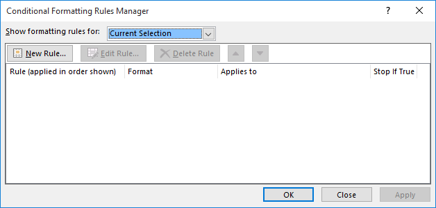
Figure 1. The Conditional Formatting Rules Manager dialog box.

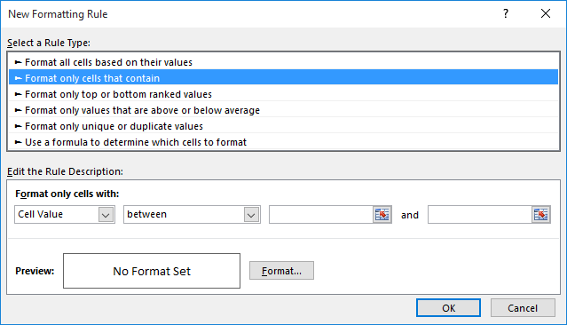
Figure 2. The New Formatting Rule dialog box.
This is a two-tiered format, and you end up with two levels of alert. If the due date is already past, then it shows up as red. If the due date is today or within the next seven days, then it shows up in blue.
ExcelTips is your source for cost-effective Microsoft Excel training. This tip (9327) applies to Microsoft Excel 2007, 2010, 2013, 2016, 2019, and 2021. You can find a version of this tip for the older menu interface of Excel here: Alerts About Approaching Due Dates.

Best-Selling VBA Tutorial for Beginners Take your Excel knowledge to the next level. With a little background in VBA programming, you can go well beyond basic spreadsheets and functions. Use macros to reduce errors, save time, and integrate with other Microsoft applications. Fully updated for the latest version of Office 365. Check out Microsoft 365 Excel VBA Programming For Dummies today!
When you paste information into a row that is conditionally formatted, you may end up messing up the rules applied to ...
Discover MoreYou can use conditional formatting to add shading to various cells in your worksheet. This tip shows how you can shade ...
Discover MoreConditional formatting allows you to change how information is displayed based on rules you define. What if you want to ...
Discover MoreFREE SERVICE: Get tips like this every week in ExcelTips, a free productivity newsletter. Enter your address and click "Subscribe."
2022-11-16 11:05:40
J. Woolley
@RB
The following three functions are included in My Excel Toolbox:
=SetFont(Name,Size,Style,Color,Underline,Strikethrough,Target)
=SetFill(Color,PatternStyle,PatternColor,Target)
=SetStyle(Name,Target)
When these functions appear in a cell formula, they will set the Target range's font, fill, or style properties. For each function, all property parameters are optional and unchanged if omitted. Target is also optional; default is the formula's cell.
These functions can be used with an IF(...) function to set or reset properties. Each function returns an empty string ("") in a text formula, zero (0) in a numeric formula, or FALSE in a boolean formula.
Here is a formula using LET (Excel 365 or 2021+) to return a Nov 16 birthday with yellow fill on Nov 16 or blank on any other day:
=LET(tday,TODAY(),bday,DATE(YEAR(tday),11,16),IF(bday=tday,SetFill("yellow")+bday,SetFill("none")&""))
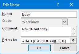
If you can't use LET, define bday as a named range (see Figure 1 below) and use this formula:
=IF(bday=TODAY(),SetFill("yellow")+bday,SetFill("none")&"")
See https://sites.google.com/view/MyExcelToolbox/

Figure 1.
2022-11-16 04:22:23
Peter Atherton
RB
Use Conditional Formatting, with fthis ormula
=DATE(YEAR(TODAY()),MONTH(B11),DAY(B11))=TODAY()
and apply your formatting
2022-11-15 06:18:55
RB
Hi
I want to high light a cell containing a date of birth only on that date. How do I go about doing this.
I want the cell to be highlighted and the text in it to be visible only on that day, the rest of the time it needs to be hidden
Any assistance will be appreciated greatly
2020-10-30 18:40:59
sara
How do I keep blank cells from turning red? I don't want the cell red or yellow unless there is a date entered.
Got a version of Excel that uses the ribbon interface (Excel 2007 or later)? This site is for you! If you use an earlier version of Excel, visit our ExcelTips site focusing on the menu interface.
FREE SERVICE: Get tips like this every week in ExcelTips, a free productivity newsletter. Enter your address and click "Subscribe."
Copyright © 2026 Sharon Parq Associates, Inc.
Comments