Filtering Addresses for a Group of States

Richard has worksheet that consists of names and addresses. The addresses are broken into separate columns, such as Street, City, State, and ZIP Code. He is interested in filtering to display only those addresses in MN, OK, IA, and IL.

There are actually several different ways you can do the filtering. Before jumping into them, though, make sure that your data has a header row; I'll assume it is in row 1.

With that said, let's take a look at five or six different approaches you can take to get the addresses you want.

Using Filtering

To filter for the desired states, you can simply select a cell within your data and, on the Data tab of the ribbon, click the Filter tool. Excel automatically adds drop-down arrows next to the column headings in the first row.

Click the drop-down arrow next to the State column and, in the resulting drop-down palette, clear the check box next to Select All. This clears all the state check boxes. Then, go through the list and select the check boxes next to MN, OK, IA, and IL. When you click on OK, only addresses in those states are displayed.

Using Advanced Filtering

To utilize advanced filtering, you need to set up a criteria table. This can be done in some unused columns to the right of your data. (Just make sure you leave one or more blank columns between your data and the criteria table.) For instance, I could set up a criteria table starting in cell J1. (See Figure 1.)

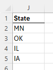
Figure 1. A simple table for advanced filtering criteria.

Notice how simple the criteria table is—all you need to do is use a heading that is the same as column heading in your data table (in this case, "State") and then list under that each state you want—you don't even need to sort the states. Then you can follow these steps:

1. Select one of the cells in your data. (Not in the criteria table.)
2. Display the Data tab of the ribbon.
3. Click the Advanced Filter tool (Excel 2007) or the Advanced tool (later versions of Excel) in the Sort & Filter group. Excel displays the Advanced Filter dialog box. (See Figure 2.)



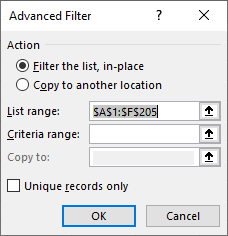
Figure 2. The Advanced Filter dialog box.

4. Make sure the "Filter the List, In Place" radio button is selected. (It probably will be, by default.)
5. The List Range should already be filled in, provided you did step 1.
6. In the Criteria Range field, specify the cells where you created your criteria table. In this example I set it to J1:J5.
7. Click on OK.

At this point, the data is filtered to display only rows having a state that matches one of the states in your criteria table.

Filtering in a Table

Another approach is to convert your data into a formal table in order to do the filtering. Just select a cell within the data and press Ctrl+T to display the Create Table dialog box. (See Figure 3.)

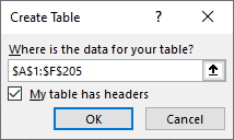
Figure 3. Creating a table.

The range of cells should automatically be added to the dialog box. Make sure the check box for "My Data Has Headers" is selected, then click on OK.

With the data in a formal table, a drop-down arrow appears next to the header row in each column. This should look familiar if you have read through this tip so far. All you need to do is to follow the same steps described earlier, under the "Using Filtering" heading. Click the drop-down arrow next to the State column, clear the check box next to Select All, then select the check boxes next to MN, OK, IA, and IL. When you click on OK, only addresses in those states are displayed.

Using a Formula

If you are using Excel 2021, Excel 2024, or Microsoft 365, you could use the FILTER function to extract the rows you want. Simply copy the column headers to a place to the right of your data; in this case, I'm going to assume that you are copying the headings from A1:F1 over to J1:O1. Then, in cell J2, place the following formula:

=FILTER(A:F,(E:E="MN")+(E:E="OK")+(E:E="IA")+(E:E="IL"))

The formula looks at the rows in columns A:F and, if column E contains one of the desired states, it returns the row.

If you want an even shorter formula and you are using Microsoft 365, then you can incorporate one of the latest regex-based functions. In that case, you would put the following formula into cell J2:

=FILTER(A:F,REGEXTEST(E:E,"^MN|OK|IA|IL$"))

The REGEXTEST function examines the values and column E (the states) and returns an array of rows that contain MN or OK or IA or IL. The vertical bar means "or," the caret means "starts with," and the dollar sign means "ends with." Thus, the function returns rows that contain only the desired two-character state names. In other words, if a state was listed as "Okla.", it wouldn't match the expression.

Using a Macro

If you wanted to use a macro to do the filtering, you could come up with one that examines the state column and if the state isn't one of the four you want, then row is hidden. Here's an example:

Sub Display_Addr()
    Dim r As Integer

    For r = 2 To Cells(Rows.Count, 5).End(xlUp).Row
        Select Case UCase(Cells(r, 5))
            Case "MN", "OK", "IA", "IL"
                Rows(r).EntireRow.Hidden = False
            Case Else
                Rows(r).EntireRow.Hidden = True
        End Select
    Next r
End Sub

The macro looks at column 5 (which is column E, in this example, the states column) and if it is one of the four desired states, then the row is displayed. Otherwise, the row is hidden. The macro runs very quickly, depending on the amount of data you have in the worksheet.

ExcelTips is your source for cost-effective Microsoft Excel training. This tip (9951) applies to Microsoft Excel 2007, 2010, 2013, 2016, 2019, 2021, 2024, and Excel in Microsoft 365.