Written by Allen Wyatt (last updated May 14, 2025)
This tip applies to Excel 2007, 2010, 2013, 2016, 2019, 2021, 2024, and Excel in Microsoft 365
Juan has a column (column A) of dates in the year 2024. He wants to copy that range of dates into another worksheet in the same workbook. He needs to make the dates all the same, except for the year, which should be 2025.
There are quite a few different ways you can go about accomplishing this task. One way is to use a formula to create the new dates. Assuming the original dates are in column A (as Juan noted) and that the worksheet is named Original Dates, you could use the following formula in cell A1 of a different worksheet:
=DATE(2025,MONTH('Original Dates'!A1),DAY('Original Dates'!A1))
You can then copy the formula down as many cells as desired. If you prefer, you can use an even shorter formula:
=EDATE('Original Dates'!A1,12)
Remember that when you use a formulaic approach, Excel may not automatically format the result to look like a date. That's easy enough to fix; just apply the cell formatting you want.
There is an important difference between the two formulas that deal with how they resolve what happens if the original date is leap day (February 29). In the case of the DATE function, Excel treats the new date as March 1. Thus, if the original date was February 29, 2024, then the result of the DATE formula would be March 1, 2025.
In the case of the EDATE function, February 29 is rendered as February 28. Thus, February 29, 2024, becomes February 28, 2025.
Whichever formula approach you use (and there are several others), once they are in place you can select all the formulas, press Ctrl+C to copy them to the Clipboard, display the Home tab of the ribbon, click the down-arrow under the Paste tool, and select to Paste Values. This does away with the formulas and leaves you with actual dates in the cells.
Speaking of copying and pasting, that brings up another way to get the dates to the new worksheet:
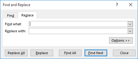
Figure 1. The Replace tab of the Find and Replace dialog box.
Excel is smart enough to know that you want to replace years, and in so doing it "reevaluates" the resulting dates. For most dates this is not a problem, but it is for leap days. If the original date is February 29, 2024, it is changed to February 29, 2025. Since that is an invalid date, it won't be correctly parsed by Excel.
There is another approach that was suggested by several ExcelTips subscribers, as follows:
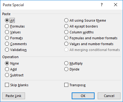
Figure 2. The Paste Special dialog box.
At first glance, it appears that all your dates are updated to be one year later than they were originally. In many instances this will be correct but, again, leap days will mess you up. If the original dates are in a year that contains a leap day, such as 2024, then adding 365 to them doesn't mean they will be a year later because the leap year contains 366 days. Thus, it is best to use one of the other methods described in this tip.
ExcelTips is your source for cost-effective Microsoft Excel training. This tip (13328) applies to Microsoft Excel 2007, 2010, 2013, 2016, 2019, 2021, 2024, and Excel in Microsoft 365.

Program Successfully in Excel! This guide will provide you with all the information you need to automate any task in Excel and save time and effort. Learn how to extend Excel's functionality with VBA to create solutions not possible with the standard features. Includes latest information for Excel 2024 and Microsoft 365. Check out Mastering Excel VBA Programming today!
Excel is great when it comes to working with dates and times. You can even do math on dates. One such easy manipulation ...
Discover MoreType a date into Excel that includes a two-digit year, and you may not always get the year in the century you intended. ...
Discover MoreWhen working with dates and the relationship between dates, Excel provides a variety of worksheet functions that may ...
Discover MoreFREE SERVICE: Get tips like this every week in ExcelTips, a free productivity newsletter. Enter your address and click "Subscribe."
2025-01-14 04:12:58
Kiwerry
@Tomek: I agree. At the end of the day, it seems to me that there is not much point in trying to format the text in a comment, unless one needs to keep part of it in one line, then non-breaking spaces come in useful. They are also, of course, very useful for formatting code so that it can be copied and pasted by users without losing the indenting.
@All: methods of replacing spaces with non-breaking spaces (hardspaces) are discussed in a number of comments below.
2025-01-13 14:10:39
Tomek
Another test, please ignore.
Interestingly, long lines without spaces in them do not break to fit in that narrow column whether on the phone or on my computer. That may be useful for posting long lines of code.
Maybe if you have spaces in the line, you can replace them with non-breaking spaces like I did in the line above.
2025-01-13 14:08:27
Tomek
@Kiwerry
It seems then that the correct width of the input window to match the actual comment display may depend on some Windows personalization settings, like fonts and their scale. So every user may find their specific mark - it is not hard to do,
I have also found that the displayed comments have much narrower column width if I read them on my Pixel 6 phone.
Interestingly, long lines without spaces in them do not break to fit in that narrow column whether on the phone or on my computer. That may be useful for posting long lines of code.
Maybe if you have spaces in the line, you can replace them with non-breaking spaces like I did in the line above.
When copying the code from the comment into VBA editor, non-breaking spaces are automatically converted into regular spaces, so this should not cause problems.
2025-01-12 18:24:20
Kiwerry
@Tomek: Thank you for yours.
I agree that it's better to use a visual clue than a measurement when resizing the comment input textbox. See fig. 1 in my comment of 2025-01-07 04:28:26,; the text in the box appeared unchanged in the relevant comment. I differ with you about which marker to use; I found the "t" in "... but an image" in the text just below the input box worked well, and have set the box to that width for this comment.
2025-01-11 00:49:01
Tomek
Now, let's get back to the topic of this tip.
The solutions provided in this tip are generally easy enough to apply, especially if you do not need to deal with the leap-year related variations. But if you do, doing it every year requires to chose which leap-year option you want, and recalling steps you did the previous year.
Rather than telling Juan how to copy and modify his data (what he asked for) I would suggest creating a workbook that generates the required column of dates (what he actually may want). This solution is based on the first tip approach (DATE formula) but rather than hard coding the year, the year can be input into a selected cell.
So here are the steps:
· Place your original dates in column A staring with cell A2.
· In cell B1 enter the target year.
· In cell B2 enter formula "=DATE(B$1,MONTH($A2),DAY($A2))"
· Copy that formula down for as many rows as you need.
A this point you should have new dates in column B, with any original Feb. 29 in leap year converted to Mar. 1 of a non-leap year. Also, Feb. 28 will stay always unchanged. If this is not what you want, you need to modify the formulas that involve Feb 28 or Feb. 29 in the original dates. You need to do this only once, afterwards you can just use the spreadsheet by entering a new target year.
You have four choices - two for Feb 28 and two for Feb 29 as original date:
· If you want Feb. 28 to always stay Feb 28 do nothing.
· If you want Feb. 28 to be treated as end of month envelop the formula in EOMONTH function: "=EOMONTH(DATE(B$1,MONTH($A4),DAY($A4)),0)"
· If you want Feb. 29 to become March 1, do nothing, the DATE function does it automatically.
· If you want Feb. 29 to be treated as end of month use EOMONTH function but subtract 1 from the day:
"= EOMONTH(DATE(B$1,MONTH($A9),DAY($A9))-1,0)"
(see Figure 1 below) a screenshot of a demo spreadsheet using this approach for combinations of normal and leap year source and target.
You can use such approach directly in your spreadsheet or if you just want explicit dates in a column you can copy the generated dates and paste them into your other spreadsheet using Paste-Special-Values followed by Paste-Special-Formats.
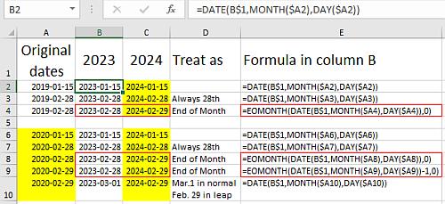
Figure 1.
2025-01-11 00:30:28
Tomek
@Kiwerry and @J. Woolley
A picture for my previous comment (see Figure 1 below)
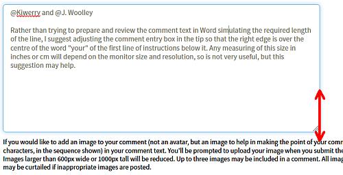
Figure 1.
2025-01-11 00:24:37
Tomek
@Kiwerry and @J. Woolley
Rather than trying to prepare and review the comment text in Word simulating the required length of the line, I suggest adjusting the comment entry box in the tip so that the right edge is over the centre of the word "your" of the first line of instructions below it. Any measuring of this size in inches or cm will depend on the monitor size and resolution, so is not very useful, but this suggestion may help.
2025-01-10 06:13:59
Kiwerry
@J. Woolley: Thanks for the tip about hardspaces causing compile errors - I knew the code copied and pasted from a comment works, but had not realised that this is because the hardspaces are replaced by spaces at some stage in the process.
2025-01-09 10:45:24
J. Woolley
@kiwerry
Transferring a Word file with non-breaking spaces to Notepad is clever.
One more thing to mention: If you have VBA code in Notepad with non-breaking spaces for indentation, copying that code from Notepad and pasting into the VB Editor (VBE) will retain the non-breaking spaces and fail to compile. In this case you must use Ctrl+H in VBE to convert groups of 4 non-breaking spaces to regular spaces. On the other hand, there is no problem when you copy VBA code from a Tip's comment into the VBE.
2025-01-09 09:03:32
kiwerry
The test code below was generated by selecting it from a website, copying it and pasting it into Word, then using Find/Replace to replace all spaces with hardspaces (which preserved the indentation and prevented long lines like the comment from wrapping), saving it as a text file, copying the text from a file viewer and pasting it here.
One could of course simply use Notepad or another editor without involving Word, which would cut out the step of saving the '.txt file, but I wanted to test a possible workaround for the problem mentioned by J. Woolley, hence the use of Word.
2025-01-09 08:50:29
kiwerry
The test was reasonably successful. On copying the code from the previous comment and pasting it into a VBA module, I found a satisfactory result.
There is a workaround for the problem of hardspaces being converted to spaces when copying text from word and pasting it into the text input box here: If the Word document is Saved As *.txt, then the hardspaces are preserved and the file can be opened with an ordinary text editor, like Notepad, copied from there and pasted into tips.net with no alteration.
2025-01-09 08:39:07
kiwerry
@J. Woolley: thank you for your most recent comment.
The following is simply a test of a possibility to post formatted VBA code here:
'============================================================================================================
Function IsDocEmpty() As Boolean
'https://answers.microsoft.com/en-us/msoffice/forum/all/word-vba-how-do-i-determine-if-the-current-word/151f4430-3868-428a-8cb5-b8ef926c846b
'============================================================================================================
Dim astory As Range
' Initialize function to True.
IsDocEmpty = True
For Each astory In ActiveDocument.StoryRanges
' Check for text. If the length of the current story is greater than one, then there is either text _
or more than one empty line.
If Len(astory.Text) > 1 Then
IsDocEmpty = False
End If
' Check for Objects.
' Note: If there are no objects within
' the current story range, an error occurs.
On Error Resume Next
If astory.ShapeRange.Count > 0 Then
If Err = 0 Then
IsDocEmpty = False
Else
On Error GoTo 0
End If
End If
' If something was found, then
' return to the calling routine with
' a value of False.
If IsDocEmpty = False Then Exit Function
Next
End Function
'============================================================================================================
2025-01-08 13:29:07
J. Woolley
@Kiwerry and Tomek
When I copy comment text samples from this Tip and paste in a Word document it uses Open Sans 11 font. If I set the margins so the text spans a width of 5.15” (13.081 cm) it appears to match the Tip’s rendering. (Margins for my 8.5”x11” paper are 1” left and 2.35” right.)
Therefore, here’s my new suggestion. Draft your comment using a Word template with those font and margin specifications, then copy it from Word and paste it into the Tip's comment entry text box. After submittal, the final result should look similar to your Word draft.
One problem with this method is that you can’t use non-breaking spaces to indent because they will be converted into standard spaces when copied from Word. Therefore, lines indented with non-breaking spaces should be drafted in Notepad and substituted in the comment entry as described in my earlier comment below.
2025-01-08 00:58:15
Tomek
@Kiwerry
On similar note, the instructions for inserting figures say that pictures wider than 600 pixels will be reduced. In fact pictures wider than 500 pixels are reduced, which degrades the quality of the pictures. You may want to keep this in mind if you want pictures of highest possible resolution.
(see Figure 1 below)
(see Figure 2 below)

Figure 1. 600 pixels wide

Figure 2. 500 pixels wide
2025-01-08 00:42:58
Tomek
@Kiwerry
Obviously my test did not quite work as I expected but it seems that 77 characters (a and o) fit in the comment width .
aaaaaoooooaaaaaoooooaaaaaoooooaaaaaoooooaaaaaoooooaaaaaoooooaaaaaoooooaaaaaoo
2025-01-08 00:36:17
Tomek
@Kiwerry
Obviously my test did not work.
2025-01-08 00:13:43
Tomek
@Kiwerry
A while ago we discussed best way to apply non-breakable spaces to format the comment text, and I guess you you still use for that. Let me know if you found something better.
As for the width of the window, what do you mean by 12 cm? Isn't that dependent on your screen size and resolution? I am going to try the next line to see how much text actually fits in the posted comment.
aaaaaoooooaaaaaoooooaaaaaoooooaaaaaoooooaaaaaoooooaaaaaoooooaaaaaoooooaaaaaoooooaaaaaoooooaaaaaoooooaaaaaoooooaaaaaoooooaaaaaoooooaaaaaoooooaaaaaoooooaaaaaoooooaaaaaoooooaaaaaoooooaaaaaooooo
Also, @J. Woolley suggestion for preparing the comment in Notepad with Verdana 11 font does not reflect exactly the font used in the comment box, nor in the posted comments. One way to tell this is to compare "g" in both fonts.
2025-01-07 12:14:49
J. Woolley
@Kiwerry
My previous comment below said, "...Notepad.exe formatted with Consolas 11 font.... Adjust the window's width to fit 79 numeric characters." Now I suggest Verdana 11 font and slightly more than 59 numeric characters (17.5 cm without the scroll bar). Consolas is a fixed font, which is good for VBA code; Verdana is a variable font, which is better for text comments.
Make sure lines indented with non-breaking spaces are preceded by CR (Enter) because word wrap can be misleading.
Here's another suggestion (which I often ignore and later regret). After preparing your draft comment in Notepad, wait another day before submitting it because you will probably think of an important change.
2025-01-07 04:28:26
Kiwerry
P.S. 10 cm was too narrow; the wrapping changed. Once I had sent the previous message I had both versions on screen and could do some experimenting. To achieve a similar wrap I had to use a width of 12 cm (see (see Figure 1 below )
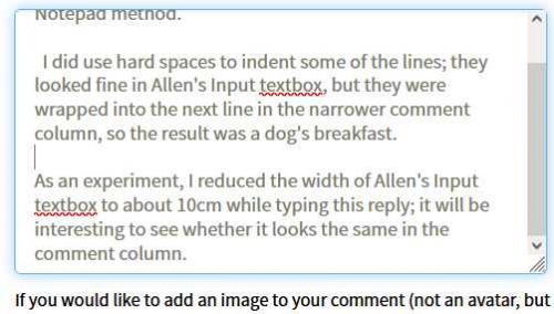
Figure 1. Input box at 12 cm wide
2025-01-07 04:14:08
Kiwerry
@ J. Woolley: Thanks very much for the tip, I'll try the Notepad method.
I did use hard spaces to indent some of the lines; they looked fine in Allen's Input textbox, but they were wrapped into the next line in the narrower comment column, so the result was a dog's breakfast.
As an experiment, I reduced the width of Allen's Input textbox to about 10cm while typing this reply; it will be interesting to see whether it looks the same in the comment column.
2025-01-06 11:35:55
J. Woolley
@Kiwerry
Re. your most recent comment below, here's my suggestion to fit "the same width as the column in which the comment will finally appear."
Prepare your comment using Windows Notepad.exe formatted with Consolas 11 font and Word Wrap. Adjust the window's width to fit 79 numeric characters. Notepad will remember these settings the next time you open it. (I'm using the Windows 10 version of Notepad. I believe there is a newer version, which might not have the same characteristics.)
For VBA code indented by 4 space characters, use Ctrl+H in Notepad to replace each group of 4 spaces with 4 non-breaking spaces. Each non-breaking space can be entered using Alt+0160 in Notepad; after one is entered, you can copy/paste it. (You can use Ctrl+Shift+Space in Word for a non-breaking space, which is visible when toggled with Ctrl+Shift+*, but non-breaking spaces are converted into standard spaces when copied from Word and pasted into another app.)
When you are satisfied with your draft comment, copy it from Notepad and paste it into the Tip's comment entry text box. After submittal, the final result should look similar to your Notepad draft.
2025-01-05 13:05:30
Kiwerry
I'll follow the comment below up with a request for Allen: if possible, please make the default width of the comment entry text box the same width as the column in which the comment will finally appear. This would allow commenters to format and space their comments better; the comment below looked fine in the text box, but after it was posted a number of lines were wrapped, making the comment more difficult to read/follow.
The comment entry text box is resizeable, but unless one knows the width of the column in which the text will ultimately be displayed that is of limited use.
2025-01-05 12:55:52
Kiwerry
Thanks for another interesting tip, Allen
I must beg to differ with your recommendation on using the Paste Special - Add method: "Thus, it is best to use one of the other methods described in this tip."
All of the methods have to deal with the change to a leap year, and the change from a leap year. They all need to deal with the fact that in the case of leap years, 366 rows are involved, not 365.
A test of the two formulae
{ slightly modified as follows:
=DATE(YEAR(A80)+Delta_Year,MONTH(A80),DAY(A80)), and
=EDATE(A80,12*Delta_Year) ,
where Delta_Year is the number of years between original and new;
if a constant value is required substitute, for example, Delta_Year by a 1 }
revealed that in changing from a leap to a non - leap year, the DATE formula results in March 1 being duplicated and the EDATE formula results in February 28 being duplicated.
In changing from a non-leap to a leap year, both omit February 29.
A test of the Paste Special, adding 365 to all values resulted in a smooth transition from the end of February into the beginning of March, no matter which direction the change took place. The problem occurs in the first row, if at all:
in changing from a leap to a non - leap year the "redundant" row is the first row; January 1 becomes 31 December of the previous year.
in changing from a non-leap to a leap year, all 366 rows are correct.
The use of the given formulae results in any event in a problem within the range; the Paste Special method results in a problem in row 1, or no problem. Take your pick.
It would of course be possible to use a formula to determine whether one of the years involved is a leap year and act accordingly. That's beyond the scope of this comment.
Got a version of Excel that uses the ribbon interface (Excel 2007 or later)? This site is for you! If you use an earlier version of Excel, visit our ExcelTips site focusing on the menu interface.
FREE SERVICE: Get tips like this every week in ExcelTips, a free productivity newsletter. Enter your address and click "Subscribe."
Copyright © 2026 Sharon Parq Associates, Inc.
Comments