Eszter has a long list of cells in column A that contain a series of mutation codes, such as "AKT 142" or "BRAF 1975." In column B are values associated with these mutation codes. She needs a formula that will sum the values in column B for which the corresponding mutation code in column A begins with the same sequence, as in all those beginning with AKT or BRAF. Eszter suspects this can be done with the SUMIF function, but she doesn't know how to make it pay attention to only the first part of the mutation code.
There are many ways you could approach this problem, but in this tip, I focus on only three potential solutions.
If your worksheet layout allows, you could add a helper column that contains only the first portion of the mutation codes. Since your mutation codes are in column A, you could insert the following formula in the first cell of your helper column:
=LEFT(A1, SEARCH(" ",A1,1)-1)
Copy it down for as many cells as necessary, and you end up with the helper column containing everything in the mutation codes before the space. You could then use your desired SUMIF formula to sum based on the contents of the helper column.
A rather unique approach to solving the problem is to use the SUMPRODUCT function. Let's say that you put, in cell E1, the preface code you are interested in. (So, for instance, you might put "AKT" into cell E1.) You could then calculate the desired sum by using the following formula:
=SUMPRODUCT(--(LEFT(A:A,LEN($E$1))=$E$1) * B:B)
This works because SUMPRODUCT examines whether the leftmost portion of a cell in column A matches whatever you put in cell E1. If it does, then the comparison returns 1; if it doesn't, it returns 0. This is then multiplied by the corresponding cell in column B and summed.
Perhaps the cleanest approach is to simply use SUMIF directly. You know, from using the helper-column approach, that you can use SUMIF to look at the contents of a cell and then selectively sum another column. You do it in this general manner:
=SUMIF(Check_Range, Criterion, Sum_Range)
Thus, if you wanted to sum values in column B based on what is in column A, you could do the following:
=SUMIF(A:A, "AKT", B:B)
This would, of course, only match those cells in column A that contain just AKT. This is not Eszter's situation, though—the mutation codes in column A contain more than just AKT. This is where the use of wildcards in the criterion specification comes into play. All Eszter needs to do is to add an asterisk, in this manner:
=SUMIF(A:A, "AKT*", B:B)
Now SUMIF returns the proper sum based only on those cells in column A that begin with the letters AKT. It doesn't matter what follows the AKT characters in each cell because the asterisk says to Excel that it should "accept anything that follows those three characters."
You could even make this approach more general in nature. Let's assume that you put the desired preface code (the one on which you want to sum) into cell E1. You could then put the following into cell E2:
=SUMIF(A:A, E1 & "*", B:B)
Now, if E1 contains "AKT" you end up with a sum of values for that preface code. If you change E1 to "BRAF" then you get a sum for that preface code, without a need to change the formula in E2.
ExcelTips is your source for cost-effective Microsoft Excel training. This tip (13614) applies to Microsoft Excel 2007, 2010, 2013, 2016, 2019, 2021, 2024, and Excel in Microsoft 365.

Excel Smarts for Beginners! Featuring the friendly and trusted For Dummies style, this popular guide shows beginners how to get up and running with Excel while also helping more experienced users get comfortable with the newest features. Check out Excel 2019 For Dummies today!
If you have circular references in a workbook, you may see an error message appear when you first open that workbook. If ...
Discover MoreYou can use the Alt+Enter keyboard shortcut while entering information in order to force your data onto multiple lines in ...
Discover MoreOperators are used in formulas to instruct Excel what to do to arrive at a result. Not all operators are evaluated in the ...
Discover MoreFREE SERVICE: Get tips like this every week in ExcelTips, a free productivity newsletter. Enter your address and click "Subscribe."
2025-01-25 01:33:26
Peter
I assume that Eszter would like a list of totals for all the mutation codes, rather than recording them one at a time. That is, to use an array of unique codes as the second argument in Sumif. nFor reasons of simplicity, format the data as a table. Change Column1 heading to "Codes" and Column2 heading to "Number". Insert one table column to the right, change its heading to "Prefix"nIn the first row under "Prefix" enter =TEXTBEFORE([@Code]]," "). You don't have to type [@Code], just click on the first value.nnIn a nearby cell enter =UNIQUE(Table1[Prefix]). In my test it was at E2. nIn a cell in an adjacent column enter =SUMIF(Table1[Prefix],E2#,Table1[Number]), Where E2 is the address of the first unique prefix in my test.nnJob done. n (see Figure 1 below)
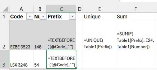
Figure 1. Formula view
2025-01-23 15:17:40
J. Woolley
Here's an interesting problem. What if the mutation codes did not have a space to separate each preface code from the remaining digits? Suppose the mutation codes were like AKT142 or BRAF1975. How would you determine the preface codes?nThe following function in My Excel Toolbox returns an array of numeric values beginning with Start incrementing by Step until Finish (not beyond):n =ForNext(Start, Finish, [Step], [AsColumn])nStart, Finish, and Step can be any numeric value. Default Step is 1.nIf AsColumn is FALSE (default), the result is a 1D row array; TRUE returns a 2D column array. Expect N elements: N = 1 + INT((Finish - Start) / Step)nUsing ForNext, this formula returns the preface code for cell A1:n =LEFT(A1, SUM(--ISERROR(VALUE(MID(A1, ForNext(1, LEN(A1)), 1)))))nMID(...) returns an array containing each character. VALUE(...) returns an error if the character is not a digit (0,1,2...). Double unary (--) converts TRUE/FALSE into 1/0. So the formula returns AKT if cell A1 is AKT142 or BRAF if it is BRAF1975.nThis formula uses the SEQUENCE function in Excel 2021 to return the same result:n =LEFT(A1, SUM(--ISERROR(VALUE(MID(A1, SEQUENCE(LEN(A1)), 1)))))nFor older versions of Excel, n SEQUENCE(LEN(A1))ncan be replaced by n ROW(INDIRECT("1:" & LEN(A1)))nMy Excel Toolbox also includes the following regular expression function:n =RegExMatch(Text, Pattern, [Mode], [IgnoreCase], [Multiline])nThis is similar to Excel's new REGEXEXTRACT function described here: https://support.microsoft.com/Search/results?query=REGEXEXTRACTnTherefore, these formulas also return the preface code for cell A1 (which is assumed to be upper case):n =RegExMatch(A1, "[A-Z]+")n =REGEXEXTRACT(A1, "[A-Z]+")nThese functions use the VBScript 5.5 regular expression syntax described here:nhttps://learn.microsoft.com/en-us/previous-versions/1400241x(v=vs.85)nOr here: https://drive.google.com/file/d/1qWS2qLib0sL_u6Sh95FuEeZxRzzr4SUE/viewnSee https://sites.google.com/view/MyExcelToolbox/
2025-01-21 15:13:21
J. Woolley
The Tip assumes the mutation codes in column A do not begin with a space and each preface code (like AKT or BRAF) ends with a space. It says, "There are many ways you could approach this problem...."nRe. Using a Helper Column:nIf column C is the helper column and the sum is desired for a preface code in cell $E$1 (which must not include a space), then use this formula:n =SUMIF(C:C, $E$1, B:B)nRe. Using SUMPRODUCT:nThis formula works just as well as the SUMPRODUCT formula:n =SUM(--(LEFT(A:A, LEN($E$1)) = $E$1) * B:B)nAgain, $E$1 must not include a space.nRe. Using SUMIF Directly:nSince the preface code ends with a space, the Tip's formulas containing an asterisk should take this into account. Therefore, they should have a space before the asterisk like this:n =SUMIF(A:A, "AKT *", B:B)n =SUMIF(A:A, $E$1 & " *", B:B)nOtherwise, there would be no difference between preface codes AKT and AKTX, for example, or between BRAF and BRAFX. As before, $E$1 must not include a space.
Got a version of Excel that uses the ribbon interface (Excel 2007 or later)? This site is for you! If you use an earlier version of Excel, visit our ExcelTips site focusing on the menu interface.
FREE SERVICE: Get tips like this every week in ExcelTips, a free productivity newsletter. Enter your address and click "Subscribe."
Copyright © 2026 Sharon Parq Associates, Inc.
Comments