Displaying Numbers as Spaced Pairs

David wonders if there is a way to format a column to display numbers as spaced pairs [xx xx xx.xx] but only display the decimal and trailing pair of a number if they exist? For instance, 123456 would display as 12 34 56 (no decimal point) and 123456.7 would display as 12 34 56.70. David cannot seem to figure this out using custom formats.

The only way to do this using custom formats is to create two custom formats. The two would look this way:

## ## ## #0
## ## ## #0.00

This would allow up to 8 digits (10 digits if you have 2 to the right of the decimal point) to be displayed as spaced pairs. The problem is that you would need to look at your data and apply whichever format is appropriate for the data. The only way to make the application of the custom formats automatic, would be to also apply conditional formatting to the cells. Once the custom formats have been defined, apply the second one (the one that allows for digits to the right of the decimal point) to all of the cells. Then follow these steps:

1. Select all the cells you want to format.
2. Make sure the Home tab of the ribbon is displayed.
3. Click the Conditional Formatting option in the Styles group. On the resulting submenu, click Manage Rules. Excel displays the Conditional Formatting Rules Manager dialog box. (See Figure 1.)



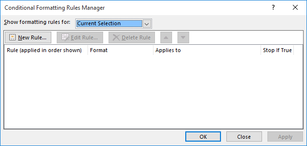
Figure 1. The Conditional Formatting Rules Manager dialog box.

4. Click the New Rule button. Excel displays the New Formatting Rule dialog box.
5. In the Select a Rule Type area at the top of the dialog box, choose Use a Formula to Determine Which Cells to Format. (See Figure 2.)



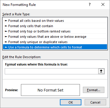
Figure 2. The New Formatting Rule dialog box.

6. In the Format Values Where This Formula Is True box, enter "=IF(A1=INT(A1),TRUE,FALSE)" (without the quote marks). The cell reference in this formula, of course, will vary depending on your data.
7. Click the Format button. Excel displays the Format Cells dialog box.
8. Using the Color drop-down list, choose the color red.
9. Click OK to close the Format Cells dialog box.
10. Display the Number tab of the ribbon.
11. At the left side of the dialog box, choose Custom.
12. In the custom formats available, choose from the custom formats you created the one that does not include anything to the right of the decimal point.
13. Click on OK to accept your formatting and to close the Format Cells dialog box.
14. Click OK. The Conditional Formatting Rules Manager dialog box reappears with your newly defined condition in it.
15. Click OK to close the Conditional Formatting Rules Manager dialog box.

Now your numbers should appear formatted just as you want them to appear.

ExcelTips is your source for cost-effective Microsoft Excel training. This tip (13771) applies to Microsoft Excel 2007, 2010, 2013, 2016, 2019, and 2021.