Please Note: This article is written for users of the following Microsoft Excel versions: 2007, 2010, 2013, 2016, 2019, 2021, and Excel in Microsoft 365. If you are using an earlier version (Excel 2003 or earlier), this tip may not work for you. For a version of this tip written specifically for earlier versions of Excel, click here: Displaying Negative Percentages in Red.
Written by Allen Wyatt (last updated October 15, 2022)
This tip applies to Excel 2007, 2010, 2013, 2016, 2019, 2021, and Excel in Microsoft 365
It's easy using Excel's built-in number formats to display negative values in red. What isn't so obvious is how to display negative percentages in red. This is because Excel doesn't provide a built-in format that addresses this situation.
There are two distinct ways you can display negative percentages in red. One way is to use a custom number format. Precise details on how you put together custom formats has been covered in other issues of ExcelTips, so here is the quick way you can get the desired results:
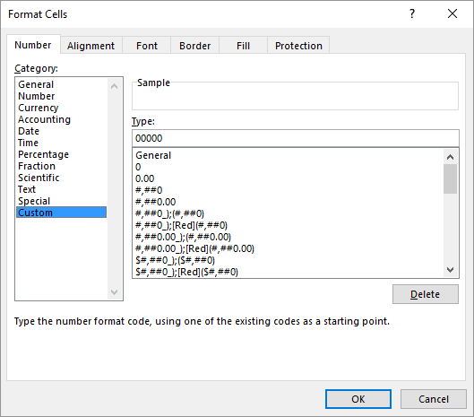
Figure 1. The Number tab of the Format Cells dialog box.
The format you specify in step 5 displays positive percentages with two decimal places and displays negative percentages in red with two decimal places. (You can modify the number of decimal places in the format, if necessary.)
The other way that you can display negative percentages in red is to use conditional formatting by following these steps:
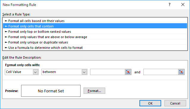
Figure 2. The New Formatting Rule dialog box.
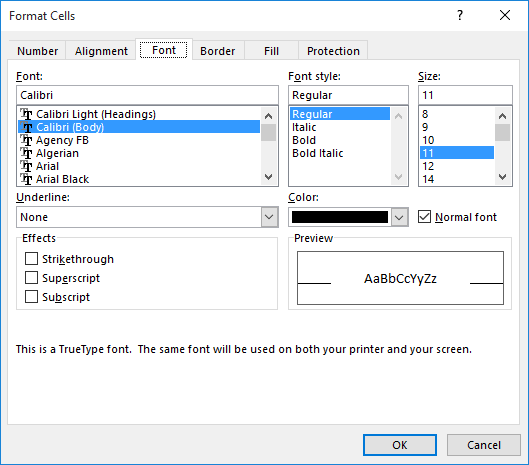
Figure 3. The Font tab of the Format Cells dialog box.
ExcelTips is your source for cost-effective Microsoft Excel training. This tip (6816) applies to Microsoft Excel 2007, 2010, 2013, 2016, 2019, 2021, and Excel in Microsoft 365. You can find a version of this tip for the older menu interface of Excel here: Displaying Negative Percentages in Red.

Solve Real Business Problems Master business modeling and analysis techniques with Excel and transform data into bottom-line results. This hands-on, scenario-focused guide shows you how to use the latest Excel tools to integrate data from multiple tables. Check out Microsoft Excel Data Analysis and Business Modeling today!
You may want Excel to format your dates using a pattern it doesn't normally use�"such as using periods instead of ...
Discover MoreExcel, by default, displays numbers with a leading zero, if they are less than 1. Here's how you can get rid of those ...
Discover MoreYou can, in a macro, specify a custom format for a range of cells. If the custom format doesn't seem to "stick" (so to ...
Discover MoreFREE SERVICE: Get tips like this every week in ExcelTips, a free productivity newsletter. Enter your address and click "Subscribe."
There are currently no comments for this tip. (Be the first to leave your comment—just use the simple form above!)
Got a version of Excel that uses the ribbon interface (Excel 2007 or later)? This site is for you! If you use an earlier version of Excel, visit our ExcelTips site focusing on the menu interface.
FREE SERVICE: Get tips like this every week in ExcelTips, a free productivity newsletter. Enter your address and click "Subscribe."
Copyright © 2025 Sharon Parq Associates, Inc.
 Please Note:
This article is written for users of the following Microsoft Excel versions: 2007, 2010, 2013, 2016, 2019, 2021, and Excel in Microsoft 365. If you are using an earlier version (Excel 2003 or earlier), this tip may not work for you. For a version of this tip written specifically for earlier versions of Excel, click here:
Please Note:
This article is written for users of the following Microsoft Excel versions: 2007, 2010, 2013, 2016, 2019, 2021, and Excel in Microsoft 365. If you are using an earlier version (Excel 2003 or earlier), this tip may not work for you. For a version of this tip written specifically for earlier versions of Excel, click here:
Comments