Finding Cells that Use Conditional Formatting

Written by Allen Wyatt (last updated June 18, 2022)
This tip applies to Excel 2007, 2010, 2013, 2016, 2019, 2021, and Excel in Microsoft 365


When you inherit a worksheet from someone, you may want to discover which cells have conditional formatting applied to them. This is rather easy to do using the Go To feature of Excel. Follow these steps:

  1. Press F5. Excel displays the Go To dialog box.
  2. Click Special. Excel displays the Go To Special dialog box. (See Figure 1.)
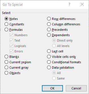
  3. Figure 1. The Go To Special dialog box.

  4. Select the Conditional Formats radio button.
  5. Click OK.

That's it. Excel selects all the cells in the current worksheet that have conditional formatting applied to them.

ExcelTips is your source for cost-effective Microsoft Excel training. This tip (6817) applies to Microsoft Excel 2007, 2010, 2013, 2016, 2019, 2021, and Excel in Microsoft 365.

Author Bio

Allen Wyatt

With more than 50 non-fiction books and numerous magazine articles to his credit, Allen Wyatt is an internationally recognized author. He is president of Sharon Parq Associates, a computer and publishing services company. ...

MORE FROM ALLEN

Jumping to a Footnote

Jumping to a specific footnote can be very handy if your document has a lot of footnotes in it. Word provides the ...

Discover More

Inserting Initials and Date in a Comment

When you insert a comment into a document, Word keeps track of who entered it and the date when it was entered. Here's ...

Discover More

Changing the Background Color for a Comment

Comments are a great way to document your worksheets. Excel provides you the tools you need in order to format your ...

Discover More

Professional Development Guidance! Four world-class developers offer start-to-finish guidance for building powerful, robust, and secure applications with Excel. The authors show how to consistently make the right design decisions and make the most of Excel's powerful features. Check out Professional Excel Development today!

More ExcelTips (ribbon)

Changing Shading when a Column Value Changes

If you have a data table in a worksheet, and you want to shade various rows based on whatever is in the first column, ...

Discover More

Working with Multiple Conditions

When you apply conditional formatting, you are not limited to using a single condition. Indeed, you can set up multiple ...

Discover More

Conditionally Highlighting Cells Containing Formulas

Excel's conditional formatting feature allows you to create formats that are based on a wide variety of criteria. If you ...

Discover More
Subscribe

FREE SERVICE: Get tips like this every week in ExcelTips, a free productivity newsletter. Enter your address and click "Subscribe."

View most recent newsletter.

Comments

If you would like to add an image to your comment (not an avatar, but an image to help in making the point of your comment), include the characters [{fig}] (all 7 characters, in the sequence shown) in your comment text. You’ll be prompted to upload your image when you submit the comment. Maximum image size is 6Mpixels. Images larger than 600px wide or 1000px tall will be reduced. Up to three images may be included in a comment. All images are subject to review. Commenting privileges may be curtailed if inappropriate images are posted.

What is 4 + 7?

There are currently no comments for this tip. (Be the first to leave your comment—just use the simple form above!)


This Site

Got a version of Excel that uses the ribbon interface (Excel 2007 or later)? This site is for you! If you use an earlier version of Excel, visit our ExcelTips site focusing on the menu interface.

Newest Tips
Subscribe

FREE SERVICE: Get tips like this every week in ExcelTips, a free productivity newsletter. Enter your address and click "Subscribe."

(Your e-mail address is not shared with anyone, ever.)

View the most recent newsletter.