Connie has a worksheet that has company names in each cell of column B. They are grouped under a region heading (Northeast, West, etc.) in column A. She would like to apply conditional formatting to the company names so that if a name appears in more than one region, it shows up using a background or text color that makes the matching companies easy to find. This means that if one company is formatted as red, no other company should appear as red (it should appear as a different color, such as blue or green). Connie isn't sure how to set this up or if it can even be done with conditional formatting.
There is a way to mark duplicates using conditional formatting; just follow these general steps:
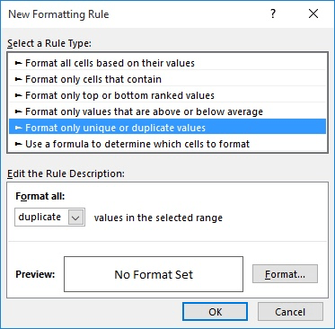
Figure 1. The New Formatting Rule dialog box.
At this point all your duplicates should match whatever formatting you selected in step 6. The only problem is that all duplicates are formatted the same way. In other words, if you have two companies (ABC Company and DEF Company) and there are duplicates for those companies, they are all formatted the same way—you won't see different formatting for the two companies.
Of course, you could easily use Excel's filtering capabilities to single out duplicate companies, non-duplicate companies, or individual company names. This might be the easiest way to "zero in" on the companies you want to locate.
The only way to use conditional formatting to apply different colors to different groups of duplicate company names requires that you identify, up front, the actual duplicates. With that list in hand, you could create a series of conditional formatting rules that use formulas similar to the following:
=AND(ISNUMBER(FIND("ABC Company",B1)),COUNTIF($B$1:$B$99,"ABC Company")>1)
In this formula "ABC Company" is the company name, B1 is the first cell of the range, and B1:B99 is the full range of cells. For each formatting rule you could apply different formatting appropriate to that particular company. That means that if you knew, up front, that there were 24 different company names that had duplicates, you would need to set up 24 conditional formatting rules to handle those 24 names.
Complex, indeed. Unfortunately, there is not an easier way using conditional formatting. You could, however, forego the conditional formatting and use a macro to make your duplicates stand out. The simplest "automatic" macro we could come up with (where you don't need to know the duplicate names ahead of time) is one that examines a range of cells and sets the internal cell color based on duplicate company names.
Sub ColorCompanyDuplicates()
    Dim x As Integer
    Dim y As Integer
    Dim lRows As Long
    Dim lColNum As Long
    Dim iColor As Integer
    Dim iDupes As Integer
    Dim bFlag As Boolean

    lRows = Selection.Rows.Count
    lColNum = Selection.Column
    iColor = 2

    For x = 2 To lRows
        bFlag = False
        For y = 2 To x - 1
            If Cells(y, lColNum) = Cells(x, lColNum) Then
                bFlag = True
                Exit For
            End If
        Next y
        If Not bFlag Then
            iDupes = 0
            For y = x + 1 To lRows
                If Cells(y, lColNum) = Cells(x, lColNum) Then
                    iDupes = iDupes + 1
                End If
            Next y
            If iDupes > 0 Then
                iColor = iColor + 1
                If iColor > 56 Then
                    MsgBox "Too many duplicate companies!", vbCritical
                    Exit Sub
                End If
                Cells(x, lColNum).Interior.ColorIndex = iColor
                For y = x + 1 To lRows
                    If Cells(y, lColNum) = Cells(x, lColNum) Then
                        Cells(y, lColNum).Interior.ColorIndex = iColor
                    End If
                Next y
            End If
        End If
    Next x
End Sub
To use the macro, simply select the cells that contain the company names and then run it. The macro makes three passes through the cells. The first pass looks backward through the cells from the current one being examined; it is used to determine if there are any "backward" duplicates, because if there are then no further processing on that particular cell is needed. The second pass looks forward through the cells to determine if there are any duplicates to the current company name. If there are, then a third pass increments the cell color value and then applies it to the duplicates.
Note that the macro sets the ColorIndex property of any duplicates it finds, and it increments the variable used to set the property when it finds a new set of duplicate company names. For all those company names for which there are no duplicates, the ColorIndex property of the cell is not changed. This means there is a limit on how many companies can be marked, however—the ColorIndex can only range between 0 and 56. The values actually assigned by the macro range from 3 to 56, so it is only possible to format 54 groupings of companies.
Note:
ExcelTips is your source for cost-effective Microsoft Excel training. This tip (12673) applies to Microsoft Excel 2007, 2010, 2013, 2016, 2019, 2021, and Excel in Microsoft 365.

Dive Deep into Macros! Make Excel do things you thought were impossible, discover techniques you won't find anywhere else, and create powerful automated reports. Bill Jelen and Tracy Syrstad help you instantly visualize information to make it actionable. You�ll find step-by-step instructions, real-world case studies, and 50 workbooks packed with examples and solutions. Check out Microsoft Excel 2019 VBA and Macros today!
If you want to highlight cells that contain certain characters, you can use the conditional formatting features of Excel ...
Discover MoreSetting up conditional formatting can be challenging under some circumstances, but once set it can work great. Unless, of ...
Discover MoreSometimes you want whatever is displayed in one cell to control what is displayed in a different cell. This tip looks at ...
Discover MoreFREE SERVICE: Get tips like this every week in ExcelTips, a free productivity newsletter. Enter your address and click "Subscribe."
2024-11-26 17:46:28
Tomek
PS: to my earlier comment. In my test spreadsheet I created a pivot table on the second sheet that also lists all unique company names along with how many times each company is listed in the data. This allows you to quickly review if a company has duplicates.
If you want to examine my spreadsheet, I suggest that you download it and open it in desktop Excel, as opening it in a browser limits available functionality of Excel and also messes up the display. To download, after opening in a browser use File - Create a Copy - Download a copy
2024-11-26 17:28:32
Tomek
This tip answered the question Connie asked, and provided some solutions to distinctly colour the relevant cells, but as Allen noted "you could easily use Excel's filtering capabilities to single out duplicate companies, non-duplicate companies, or individual company names. This might be the easiest way to "zero in" on the companies you want to locate."
I am going to suggest to take this approach a step further, and I suggest using a relatively new Excel feature to make analyzing this kind of data very easy. This feature is Slicer and once you learn to use it, I bet you will make it one of your "own" tools.
One of the ways Slicer works is using data in an Excel table, so once you have your data you can convert it to a table using "Format as a table" on the Home tab. Before you do that, it is a good practice to add a column with consecutive numbers next to your data; this will help to restore the original order of the records in case you change it by sorting. When converting to a table, make sure to check "My data has headers" in the Create-Table dialog box. I suggest using a relatively plain table formatting style for this particular scenario.
Once you have your data in Excel table, place the cursor in any of the table cells, and on the Table Design tab select insert Slicer. Select Company Name for the slicer to use, and press OK. The slicer appears with all company names selected. You can click on any Company Name and the display will show only the rows for the company selected. You can select several companies at once with Ctrl+click, or activate Multi select by clicking an icon on the top of slicer. The other icon removes the filter and selects all companies.
You should keep the slicer close to the top of the sheet and to the columns of data for ease of use.
The company choices in the slicer are only unique names arranged alphabetically. Multiple selection allows showing companies that differ by only the suffix in the name like Rise Automation Plus, Ltd and Rise Automation Plus, GmbH, as they will be next to each other in the slicer.
The slicer operates by setting the filter for the table so you can modify and sort the table using the filter button for columns in the table.
For the example screenshots of my test workbook (see Figure 1 below) and (see Figure 2 below)
You may also view and download my test worksheet from:
https://1drv.ms/x/c/bcedd6ef53b6107c/ERKW9p0BLCVJlaVTR3c7uFoBA8TRbJGdKMe6p7S-yehSfQ?e=D0kjev
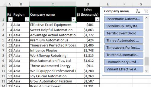
Figure 1.
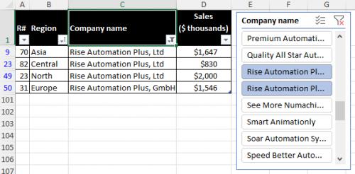
Figure 2.
2024-11-26 13:01:56
J. Woolley
The Tip's macro has several issues:
1. It picks from the 56 color current palette, which is usually the same as the default palette. The first 2 colors (black and white) are skipped, leaving 54. But 10 colors in the default palette are duplicates, so only 44 of the 54 are unique. Therefore, duplicated companies with different names might have the same color.
2. It treats text, numeric, logical, and blank values the same, so cells without names might receive a fill color.
3. It does not reset each cell's default fill color.
4. It does not adjust font color, so the text of some names might be obscured by the cell's fill color.
5. It will run a very long time if Connie selects the entire column instead of limiting the selection to names.
The following version resolves these issues. It uses a VBA Collection object for improved efficiency (only one pass through the cells).
Sub ColorCompanyDuplicates2()
Dim rCells As Range, rCell As Range, rItem As Range
Dim cNames As New Collection, sName As String, vItem As Variant
Dim bDup As Boolean, nFill As Integer, nFont As Integer, nRGB As Long
Const BLACK = 1, WHITE = 2 'ColorIndex
On Error Resume Next
Set rCells = Application.Intersect(Selection, ActiveSheet.UsedRange)
If Err <> 0 Then Exit Sub
If rCells.Cells.Count < 2 Then Exit Sub
On Error GoTo 0
nFill = WHITE
For Each rCell In rCells
vItem = VBA.Array(xlColorIndexNone, xlColorIndexAutomatic) 'default
If WorksheetFunction.IsText(rCell.Value) And rCell.Value <> "" Then
sName = rCell.Value
On Error Resume Next
cNames.Add rCell, sName 'cell is item, name is key
bDup = (Err <> 0) 'True if duplicate name
On Error GoTo 0
If bDup Then 'name is duplicate
If TypeOf cNames.Item(sName) Is Range Then 'new duplicate
Set rItem = cNames.Item(sName) 'first cell with name
nFill = nFill + 1
If nFill > 56 Then
MsgBox "Too many duplicate names!", vbCritical
Exit Sub
End If
Select Case nFill 'skip default palette's repeated colors
Case 25: nFill = 33
Case 34: nFill = 35
Case 54: nFill = 55
End Select
rItem.Interior.ColorIndex = nFill
nRGB = rItem.Interior.Color 'ColorIndex's RGB value
nFont = IIf(Round(Darkness(nRGB), 2) < 0.5, BLACK, WHITE)
rItem.Font.ColorIndex = nFont
vItem = VBA.Array(nFill, nFont)
cNames.Remove sName 'done with rItem for name
cNames.Add vItem, sName 'replace rItem with vItem
Else 'more than 2 cells with same name
vItem = cNames.Item(sName) 'fill and font for that name
End If
End If
End If
rCell.Interior.ColorIndex = vItem(0) 'fill color
rCell.Font.ColorIndex = vItem(1) 'font color
Next rCell
End Sub
Function Darkness(ColorRGB As Long) As Single
'Return the relative darkness of a ColorRGB value as
' a decimal number between 0 (white) and 1 (black)
'See https://stackoverflow.com/questions/596216
Dim Red As Integer, Green As Integer, Blue As Integer
Dim Brightness As Single
Red = (ColorRGB Mod 256)
Green = (ColorRGB \ 256) Mod 256
Blue = (ColorRGB \ 65536) Mod 256
Brightness = 0.2126 * Red + 0.7152 * Green + 0.0722 * Blue
Darkness = (255 - Brightness) / 255
End Function
If Connie adds or deletes a company name, she should run the macro again. If any names are calculated values instead of constants, she should run it each time the worksheet is calculated.
For more about Windows colors, see my comment dated 2024-07-05 here:
https://excelribbon.tips.net/T009092#comment-form-hd
Got a version of Excel that uses the ribbon interface (Excel 2007 or later)? This site is for you! If you use an earlier version of Excel, visit our ExcelTips site focusing on the menu interface.
FREE SERVICE: Get tips like this every week in ExcelTips, a free productivity newsletter. Enter your address and click "Subscribe."
Copyright © 2026 Sharon Parq Associates, Inc.
Comments