Please Note: This article is written for users of the following Microsoft Excel versions: 2007, 2010, 2013, 2016, 2019, 2021, and Excel in Microsoft 365. If you are using an earlier version (Excel 2003 or earlier), this tip may not work for you. For a version of this tip written specifically for earlier versions of Excel, click here: Shading Rows with Conditional Formatting.
Written by Allen Wyatt (last updated July 8, 2023)
This tip applies to Excel 2007, 2010, 2013, 2016, 2019, 2021, and Excel in Microsoft 365
If you haven't tried out the conditional formatting features of Excel before, they can be quite handy. One way to use this feature is to cause Excel to shade every other row in your data. This is great when your data uses a lot of columns and you want to make it a bit easier to read on printouts. Simply follow these steps:
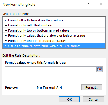
Figure 1. The New Formatting Rule dialog box.
=MOD(ROW(),2)=0
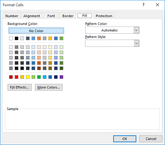
Figure 2. The Fill tab of the Format Cells dialog box.
You may wonder why anyone would use conditional formatting to highlight different rows of a table when you can use the table formatting feature (available in the Styles group of the Home tab of the ribbon) to accomplish the same thing. The reason is simple—using conditional formatting provides much more flexibility in the formatting applied as well as in the interval of the rows being shaded.
Note:
ExcelTips is your source for cost-effective Microsoft Excel training. This tip (7363) applies to Microsoft Excel 2007, 2010, 2013, 2016, 2019, 2021, and Excel in Microsoft 365. You can find a version of this tip for the older menu interface of Excel here: Shading Rows with Conditional Formatting.

Professional Development Guidance! Four world-class developers offer start-to-finish guidance for building powerful, robust, and secure applications with Excel. The authors show how to consistently make the right design decisions and make the most of Excel's powerful features. Check out Professional Excel Development today!
Need to have your worksheet printout start on a new page every time a value in a column changes? There are a couple of ...
Discover MoreIf you have conditional formatting applied in a worksheet, the formulas in those formats may not be as secure as you ...
Discover MoreExcel's conditional formatting feature allows you to create formats that are based on a wide variety of criteria. If you ...
Discover MoreFREE SERVICE: Get tips like this every week in ExcelTips, a free productivity newsletter. Enter your address and click "Subscribe."
2023-07-11 03:56:45
Enno
OK. I thought, that "shading" is a sort of darker line around the cells.
Yes, I am old enough to remember these papers.
2023-07-10 06:09:00
Steve Jez
Enno,
IMO there is no real difference, shading is generally used to identify rows that are coloured to assist "reading" data, where the data extends across a number of columns. Generally a lighter colour is used in these situations so as not to be too distracting.
If you're old enough, think of the green & white fan fold printer paper of the 80's used in the dot matrix printers.
2023-07-10 02:31:19
Enno
Can you tell me, what the difference is between "to fill" and "to shade".?
I used the description here and got cells, that are completely filled with the used color. Where ist the "shade"?
EPG
2023-07-08 05:01:31
Steve Jez
If you just need to shade alternate rows then you could use
=ISEVEN(ROW()) or =ISODD(ROW())
you can then use whichever suits your first shaded row.
Got a version of Excel that uses the ribbon interface (Excel 2007 or later)? This site is for you! If you use an earlier version of Excel, visit our ExcelTips site focusing on the menu interface.
FREE SERVICE: Get tips like this every week in ExcelTips, a free productivity newsletter. Enter your address and click "Subscribe."
Copyright © 2025 Sharon Parq Associates, Inc.
 Please Note:
This article is written for users of the following Microsoft Excel versions: 2007, 2010, 2013, 2016, 2019, 2021, and Excel in Microsoft 365. If you are using an earlier version (Excel 2003 or earlier), this tip may not work for you. For a version of this tip written specifically for earlier versions of Excel, click here:
Please Note:
This article is written for users of the following Microsoft Excel versions: 2007, 2010, 2013, 2016, 2019, 2021, and Excel in Microsoft 365. If you are using an earlier version (Excel 2003 or earlier), this tip may not work for you. For a version of this tip written specifically for earlier versions of Excel, click here:
Comments