Removing Duplicates Based on a Partial Match

Farris has a worksheet that contains addresses. Some addresses are very close to the same, such that the street address is the same and only the suite number portion of the address differs. For instance, one row may have an address of "85 Seymour Street, Suite 101" and another row may have an address of "85 Seymour Street, Suite 412." Farris is wondering how to remove the duplicates in the list of addresses based on a partial match—based only on the street address and ignoring the suite number.

The simplest solution is to further split the addresses into separate columns, such that the suite number is in its own column. You can do that by following these steps:

1. Make sure there is a blank column to the right of the address column.
2. Select the cells that contain addresses.
3. Display the Data tab of the ribbon.
4. Click the Text to Columns tool in the Data Tools group. Excel starts the Convert Text to Columns wizard. (See Figure 1.)



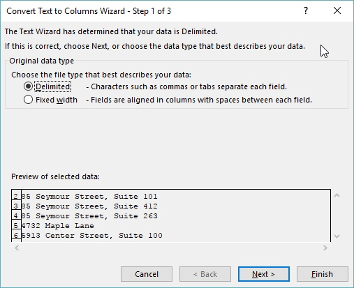
Figure 1. The Convert Text to Columns wizard.

5. In the first step of the Wizard, make sure the Delimited option is selected, then click Next.
6. In the second step of the Wizard, make sure the Comma check box is selected, then click Next.
7. In the third step of the Wizard click Finish.

The street address should now reside in the original column and the previously blank column should now contain everything that was after the comma in the original addresses. In other words, the suite number is in its own column. With your data in this condition it is an easy step to use filtering to display or extract the unique street addresses.

If you don't want to permanently split up the addresses into two columns, you could use a formula to determine duplicates. Assuming that the address list is sorted, you could use a formula similar to the following:

=IF(OR(ISERROR(FIND(",",A3)),ISERROR(FIND(",",A2))),
"",IF(LEFT(A3,FIND(",",A3))=LEFT(A2,FIND(",",A2)),
"Duplicate",""))

This formula assumes that the addresses to be checked are in column A and that this formula is placed somewhere in row 3 of a different column. It first checks if there is a comma in either the address in the current row or the address in the row before. If there is no comma in either of the addresses, then it assumes there is no possible duplicate. It there is a comma in both of them, the formula checks the portion of the addresses before the comma. If they match, then the word "Duplicate" is returned; if they don't match, then nothing is returned.

The result of copying the formula down the column (so that one formula corresponds to each address) is that you will have the word "Duplicate" appear next to those addresses which match the first part of the previous address. You can then figure out what you want to do with those duplicates that are found.

Another option is to use a macro to determine your possible duplicates. There are any number of ways that a macro to determine duplicates could be devised; the one shown here simply checks the first X characters of a "key" value against a range and returns the address of the first matching cell.

Function NearMatch(vLookupValue, rng As Range, iNumChars)
    Dim x As Integer
    Dim sSub As String

    Set rng = rng.Columns(1)
    sSub = Left(vLookupValue, iNumChars)
    For x = 1 To rng.Cells.Count
        If Left(rng.Cells(x), iNumChars) = sSub Then
            NearMatch = rng.Cells(x).Address
            Exit Function
        End If
    Next
    NearMatch = CVErr(xlErrNA)
End Function

For instance, let's assume that your addresses are in the range A2:A100. In column B you can use this NearMatch function to return addresses of possible duplicates. In cell B2 enter the following formula:

=NearMatch(A2,A3:A$100,12)

The first parameter for the function (A2) is the cell you want to use as your "key." The first 12 characters of this cell are compared against the first 12 characters of each cell in the range A3:A$100. If a cell is found in that range in which the first 12 characters match, then the address of that cell is returned by the function. If no match is located, then the #N/A error is returned. If you copy the formula in B2 down, to cells B3:B100, each corresponding address in column A is compared to all the addresses below it. You end up with a list of possible duplicates in the original list.

ExcelTips is your source for cost-effective Microsoft Excel training. This tip (7886) applies to Microsoft Excel 2007, 2010, 2013, 2016, 2019, Excel in Microsoft 365, and 2021. You can find a version of this tip for the older menu interface of Excel here: Removing Duplicates Based on a Partial Match.