Filtering Based on Comparing Two Cells

Hank has a worksheet in which he tracks various items manufactured by his company. One of the columns contains an estimated cost for each item, and another column contains the actual cost of the item. There are about 1500 rows of data in the worksheet, and it would be very helpful for Hank if he could filter the data to show just the rows where the actual cost differs from the estimated cost.

There are several ways that this can be done. The traditional approach is to add a simple helper column to detail the difference between the two columns. Assuming that your estimated cost is in column C and your actual cost is in column D, then you could place the following formula in each cell of the helper column:

=C1-D1

What you end up with is a column that shows the variance between actual and estimated costs. You can then filter based on the helper column, which allows you to display only the rows you want.

Of course, this is a sneaky way of getting around the desire to filter based on the comparison of two cells—your helper column is, after all, a single cell on which you are filtering. You could, continue this sneaky approach, however, by using a variation that doesn't require the helper column. Apply a conditional format to the cells in column D (the actual cost) that highlights the cell in one color if the actual cost is below the estimated and a different color if it is above the estimated. With the colors showing, you could then easily filter based on the colors, again giving you just the rows you want to see.

A third approach is to utilize an advanced filter to limit your rows. Again, I'm assuming that your estimated cost is in column C (cells C2:C1501) and the actual cost is in column D (cells D2:D1501). Each cell in row 1 should have a column header, such as "Estimated" and "Actual." Now you need to create a small criteria table, somewhere in an unused area of your worksheet. In this case, I entered the word "Difference" into cell K1 and the following formula into cell K2:

=C2<>D2

The word I entered into cell K1 didn't really matter; it was necessary because the Advanced Filter tool expects a header in the criteria table. The key is the formula entered into cell K2. With the criteria table in place, I then followed these steps:

1. Select any cell in the original data table (not in the criteria table).
2. Display the Data tab of the ribbon.
3. Click Advanced in the Sort & Filter group. Excel displays the Advanced Filter dialog box, with the address of your original data table already filled in, in the List Range box. (See Figure 1.)



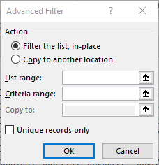
Figure 1. The Advanced Filter dialog box. Your data range shown will be different.

4. Select the Criteria Range field. The insertion point should appear within the field.
5. Use the mouse to select the criteria range, cells K1:K2.
6. Click on OK.

That's it. Excel immediately filters your data to show only those rows where the actual cost differs from the estimated cost.

A fourth approach can be used if two conditions are met. First, that you have your data range formatted as a table and, second, that you are using Excel 2021 or the version of Excel provided with Office 365. Then all you would need to do is to find an unused area of your worksheet and enter the following formula:

=FILTER(Table1,Table1[Actual]<>Table1[Estimated],"")

The formula spills into as many cells as necessary in order to return the rows where the actual and estimated costs differ. This approach is very simple, and I only noted two potential drawbacks. First, the FILTER function does not return column headings; it just returns data rows. The second potential drawback is that it always returns something, even if there was nothing in some of the source cells. For instance, if you have a column in your data called Comments, and there is not a comment in every cell in the column, then FILTER returns a 0 value for those empty cells. These two potential drawbacks can make your returned data look a little funky, but that can always be touched up with the judicious use of formatting.

ExcelTips is your source for cost-effective Microsoft Excel training. This tip (12924) applies to Microsoft Excel 2007, 2010, 2013, 2016, 2019, Excel in Microsoft 365, and 2021.