Please Note: This article is written for users of the following Microsoft Excel versions: 2007, 2010, 2013, 2016, 2019, and 2021. If you are using an earlier version (Excel 2003 or earlier), this tip may not work for you. For a version of this tip written specifically for earlier versions of Excel, click here: Using List Box Controls.
Written by Allen Wyatt (last updated December 27, 2022)
This tip applies to Excel 2007, 2010, 2013, 2016, 2019, and 2021
Excel allows you to define graphical controls within your worksheet. Buttons and other controls are placed in your worksheet by displaying the Developer tab of the ribbon and using the Insert tool in the Controls group.
One of the form controls you can place in your worksheet is called a list box. This is a scrollable list of options from which the user can choose. You might use these in a worksheet if you have a group of options from which you want the user to choose. Let's assume you have a worksheet that provides a price quote and the price is contingent on which color of widget the user wants. Having the users type the name of a color is open to error. For instance, they might enter the name of a color you don't carry, misspell the color name, or refer to a color as "gray" when your terminology is "slate." Rather than have them type a color in, you can present the various colors in a list from which they can choose.
To place a list box control in your worksheet, display the Developer tab of the ribbon, click the Insert tool (in the Controls group), and then click the List Box tool in the Form Controls section. You then use the mouse to define the rectangle that will hold the list box and the scroll bar at the right side of the box.
To use a list box effectively, you have to link it to two separate areas on your worksheet. The first is called an input list, and represents the options in the list. The second is the cell link, which contains the currently selected option. To set these areas, follow these steps:
You should note that the Cell Link setting specifies a bi-directional relationship between the cell and the control. This means that a change in the selected option will change the value in the cell, but a change in the cell value will also change which option is selected in the list box. The value stored in the linked cell indicates the number of the option selected in the list. Thus, if you have a list of seven options and the second option in the list is selected, the value in the linked cell will be 2.
ExcelTips is your source for cost-effective Microsoft Excel training. This tip (8318) applies to Microsoft Excel 2007, 2010, 2013, 2016, 2019, and 2021. You can find a version of this tip for the older menu interface of Excel here: Using List Box Controls.

Create Custom Apps with VBA! Discover how to extend the capabilities of Office 365 applications with VBA programming. Written in clear terms and understandable language, the book includes systematic tutorials and contains both intermediate and advanced content for experienced VB developers. Designed to be comprehensive, the book addresses not just one Office application, but the entire Office suite. Check out Mastering VBA for Microsoft Office 365 today!
Lots of people prefer to enter information directly into Excel, but there is another way that may be helpful: Using data ...
Discover MoreForm controls can be a great way to get information into a worksheet. They are designed to be linked to a cell so that ...
Discover MoreRadio buttons are great for some data collection purposes. They may not be that great for some purposes, however, for the ...
Discover MoreFREE SERVICE: Get tips like this every week in ExcelTips, a free productivity newsletter. Enter your address and click "Subscribe."
2022-12-29 07:56:26
Mike J
This tip looks like a solution desperately looking for a problem to solve, and it is not even reliable.
For example, this is a "bi-directional relationship", so if you have a list of say, 7 items, and then type in '9', there is no error message, the list now just exhibits the last (7th) item.
Also, if you re-sort the list after selecting it from the drop-down box, the selection may well change, and no longer be correct.
It's difficult to see how this solution improves on the much simpler Data Validation/List method, which does not seem to suffer from these potential errors.
2022-12-27 14:20:39
Ken Kast
Allen, It's been helpful that you added the "applies to" caveat at the top of a tip. It turns out, tho, that a fair number of your tips apply only to Excel (Microsoft 365) on the Windows platform. We Mac users are left searching in vain. Today's tip is an example. Could you expand your "applies to" to include whether it's for all platforms or Windows only? Thanks.
2022-12-27 10:32:55
Bruce Watson
When using the List Box, the Output to the designated cell is a Number, not the selected text. 1st item in list returns "1", second item returns "2" and so on... Would one need to set a Vlookup table and formula to return the text entry selected instead of the position number in the list?
(see Figure 1 below)
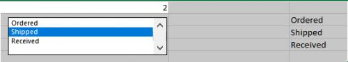
Figure 1. Screen Shot
Got a version of Excel that uses the ribbon interface (Excel 2007 or later)? This site is for you! If you use an earlier version of Excel, visit our ExcelTips site focusing on the menu interface.
FREE SERVICE: Get tips like this every week in ExcelTips, a free productivity newsletter. Enter your address and click "Subscribe."
Copyright © 2025 Sharon Parq Associates, Inc.
 Please Note:
This article is written for users of the following Microsoft Excel versions: 2007, 2010, 2013, 2016, 2019, and 2021. If you are using an earlier version (Excel 2003 or earlier), this tip may not work for you. For a version of this tip written specifically for earlier versions of Excel, click here:
Please Note:
This article is written for users of the following Microsoft Excel versions: 2007, 2010, 2013, 2016, 2019, and 2021. If you are using an earlier version (Excel 2003 or earlier), this tip may not work for you. For a version of this tip written specifically for earlier versions of Excel, click here:
Comments