Please Note: This article is written for users of the following Microsoft Excel versions: 2007, 2010, 2013, 2016, 2019, and 2021. If you are using an earlier version (Excel 2003 or earlier), this tip may not work for you. For a version of this tip written specifically for earlier versions of Excel, click here: Merging Cells to a Single Sum.
Written by Allen Wyatt (last updated April 18, 2024)
This tip applies to Excel 2007, 2010, 2013, 2016, 2019, and 2021
As you analyze your data in a worksheet, one common task is to look for ways to simplify the amount of data you need to work with. One way to do this is to "merge" several consecutive cells together in an Excel worksheet, leaving only the sum of the original cells as a value. For instance, if you have values in the range B3:F3, how would you collapse the range into a single cell that contains just the sum of that range?
The easiest way I have found to accomplish this task is as follows:
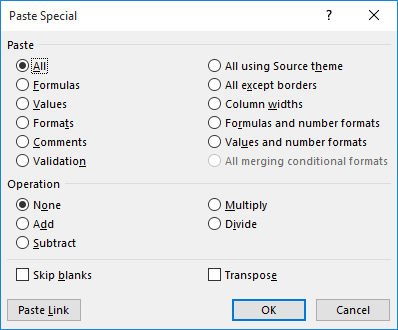
Figure 1. The Paste Special dialog box.
When you clicked the down-arrow under the Paste tool (in step 7), you may have noticed a number of different choices you could make. If you don't want to display the Paste Special dialog box, you could instead click the Values option in the Paste Values section of the drop-down list. The Values option is the left-most option in the Paste Values section; it looks like a clipboard with the number 123 on it.
ExcelTips is your source for cost-effective Microsoft Excel training. This tip (9146) applies to Microsoft Excel 2007, 2010, 2013, 2016, 2019, and 2021. You can find a version of this tip for the older menu interface of Excel here: Merging Cells to a Single Sum.

Excel Smarts for Beginners! Featuring the friendly and trusted For Dummies style, this popular guide shows beginners how to get up and running with Excel while also helping more experienced users get comfortable with the newest features. Check out Excel 2019 For Dummies today!
Separating text values in one cell into a group of other cells is a common need when dealing with text. Excel provides a ...
Discover MoreDo you need to know how many words are in a range of cells? Excel provides no intrinsic way to count the words, but you ...
Discover MoreWant a quick way to tell how may rows and columns you've selected? Here's what I do when I need to know that information.
Discover MoreFREE SERVICE: Get tips like this every week in ExcelTips, a free productivity newsletter. Enter your address and click "Subscribe."
There are currently no comments for this tip. (Be the first to leave your comment—just use the simple form above!)
Got a version of Excel that uses the ribbon interface (Excel 2007 or later)? This site is for you! If you use an earlier version of Excel, visit our ExcelTips site focusing on the menu interface.
FREE SERVICE: Get tips like this every week in ExcelTips, a free productivity newsletter. Enter your address and click "Subscribe."
Copyright © 2025 Sharon Parq Associates, Inc.
 Please Note:
This article is written for users of the following Microsoft Excel versions: 2007, 2010, 2013, 2016, 2019, and 2021. If you are using an earlier version (Excel 2003 or earlier), this tip may not work for you. For a version of this tip written specifically for earlier versions of Excel, click here:
Please Note:
This article is written for users of the following Microsoft Excel versions: 2007, 2010, 2013, 2016, 2019, and 2021. If you are using an earlier version (Excel 2003 or earlier), this tip may not work for you. For a version of this tip written specifically for earlier versions of Excel, click here:
Comments