Pulling Apart Cells

It's probably happened to you before: you get data for your worksheet, and one of the columns includes names. The only problem is the names are all bunched together. For instance, the cell contains "Allen Wyatt," but you would rather have the first name in one column, and the last name in the neighboring column to the right. How do you pull the names apart?

You can easily use the Text to Columns feature in Excel to pull your data apart. Just follow these steps:

1. Select the range of cells you want to split.
2. Display the Data tab of the ribbon.
3. Click the Text to Columns tool, in the Data Tools group. Excel starts the Convert Text to Columns Wizard. (See Figure 1.)



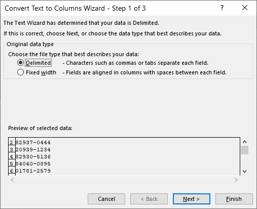
Figure 1. The beginning of the Convert Text to Columns Wizard.

4. Choose whether the text you have selected is fixed width or delimited. (In the case of a space between first and last name, the text would be delimited.)
5. Click on Next.
6. Specify the delimiters you want Excel to recognize. In the case of pulling apart names, you should make sure that you use spaces as delimiters.
7. Click on Finish.

Excel pulls apart the cells in your selected range, separating all the text at the delimiter you specified. Excel uses however many columns are necessary to hold the data. (Make sure you have blank columns to the right of the one you are splitting. If you don't, you could easily overwrite data already in those columns.)

If you don't want to spread your data completely across the columns, then you will need to use a macro. For instance, if a cell contains "John Davis, Esq.", then using the Text to Columns feature will result in the data being spread into three columns: the first containing "John", the second containing "Davis," (with the comma), and the third containing "Esq." If you would rather have the data split into two columns ("John" in one and "Davis, Esq." in the other, then the following macro will be helpful:

Sub PullApart()
    Dim Cell As Range
    Dim k As Integer

    For Each Cell In Selection
        k = InStr(Cell, " ")
        If k Then
            Cell.Offset(0, 1) = Mid(Cell, k + 1)
            Cell = Left(Cell, k - 1)
        End If
    Next
End Sub

This macro examines each cell and leaves everything up to the first space in the selected cell and moves everything after the space into the column to the right. The only "gottcha" with this macro is to make sure you have nothing in the column to the right of whatever cells you select when you run it.

ExcelTips is your source for cost-effective Microsoft Excel training. This tip (9932) applies to Microsoft Excel 2007, 2010, 2013, 2016, 2019, 2021, 2024, and Excel in Microsoft 365. You can find a version of this tip for the older menu interface of Excel here: Pulling Apart Cells.