Freezing Top Rows and Bottom Rows

Kevin has a long (vertical) worksheet that has the first few rows frozen so the column headings are always visible. He would like to also freeze the bottom row, so the column totals are always visible.

Unfortunately there is no way to do this in Excel. At first thought you may believe that you can freeze rows and also split the worksheet window so that you can put the totals below the split. Excel won't let you do this, however—when you try, then the freeze is removed and replaced with the split, and trying to reapply the freeze removes the split.

What most experienced Excel users do is to put the column totals at the top of the columns instead of at the bottom. This may seem awkward, but it has the added benefit of allowing you to easily add new rows to your data table. The top-of-column totals could be added either using SUM formulas (as you would with the totals at the bottom), or you can leave the totals at the bottom of the columns and simply add a referential formula (like =B327) in a row at the top of columns.

There is another approach you can use, however. Start by opening the workbook that contains the worksheet you want to work on. (This should be the only workbook open.) Then follow these steps:

1. Display the View tab of the ribbon.
2. Click the New Window tool in the Window group. Excel creates a new window on the data in the worksheet you are working on.
3. Click the Arrange All tool in the Window group. You should see the Arrange Windows dialog box. (See Figure 1.)



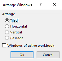
Figure 1. The Arrange Windows dialog box.

4. Make sure the Horizontal radio button is selected.
5. Click OK.

At this point you should see your two windows—one in the top half of the screen and the other beneath it. Use the mouse to adjust the vertical height of both windows. (The bottom window should be large enough to hold your totals and the top window can occupy the rest of the available space.)

Now you can display the totals row (or rows) in the bottom window, and freeze the top rows in the top window. This allows you to see everything you want to see, although it is a bit expensive when it comes to screen real estate since both windows have column letters visible.

The biggest drawback to this approach is that the windows are not horizontally linked. This means that if you scroll one of the windows left or right, the other window doesn't scroll at the same time. You could write some VBA code to handle the horizontal scrolling, but that simply adds complexity to the situation.

ExcelTips is your source for cost-effective Microsoft Excel training. This tip (9841) applies to Microsoft Excel 2007, 2010, 2013, 2016, 2019, 2021, and Excel in Microsoft 365. You can find a version of this tip for the older menu interface of Excel here: Freezing Top Rows and Bottom Rows.