Please Note: This article is written for users of the following Microsoft Excel versions: 2007, 2010, 2013, 2016, 2019, and 2021. If you are using an earlier version (Excel 2003 or earlier), this tip may not work for you. For a version of this tip written specifically for earlier versions of Excel, click here: Conditionally Highlighting Cells Containing Formulas.
Written by Allen Wyatt (last updated January 23, 2021)
This tip applies to Excel 2007, 2010, 2013, 2016, 2019, and 2021
You probably already know that you can select all the cells containing formulas in a worksheet by pressing F5 and choosing Special | Formulas. If you need to keep a constant eye on where formulas are located, then repeatedly doing the selecting can get tedious. A better solution is to use the conditional formatting capabilities of Excel to highlight cells with formulas.
Before you can use conditional formatting, however, you need to create a user-defined function that will return True or False, depending on whether there is a formula in a cell. The following macro will do the task very nicely:
Function HasFormula(rCell As Range) As Boolean
    Application.Volatile
    HasFormula = rCell.HasFormula
End Function
To use this with conditional formatting, select the cells you want checked, and then follow these steps:
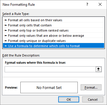
Figure 1. The New Formatting Rule dialog box.
Microsoft introduced the ISFORMULA function with Excel 2013. The ISFORMULA function allows you to highlight cells that contain formulas without using a macro. To use this function with conditional formatting, select the cells you want checked, and then follow these steps:
Note:
ExcelTips is your source for cost-effective Microsoft Excel training. This tip (9900) applies to Microsoft Excel 2007, 2010, 2013, 2016, 2019, and 2021. You can find a version of this tip for the older menu interface of Excel here: Conditionally Highlighting Cells Containing Formulas.

Create Custom Apps with VBA! Discover how to extend the capabilities of Office 365 applications with VBA programming. Written in clear terms and understandable language, the book includes systematic tutorials and contains both intermediate and advanced content for experienced VB developers. Designed to be comprehensive, the book addresses not just one Office application, but the entire Office suite. Check out Mastering VBA for Microsoft Office 365 today!
Conditional formatting is a great tool. You may need to use this tool to tell the difference between cells that are empty ...
Discover MoreYou can use conditional formatting to add shading to various cells in your worksheet. This tip shows how you can shade ...
Discover MoreNeed to know if a particular cell contains a date value? Excel doesn't have a worksheet function to determine this ...
Discover MoreFREE SERVICE: Get tips like this every week in ExcelTips, a free productivity newsletter. Enter your address and click "Subscribe."
2021-01-25 14:23:54
J. Woolley
You might be interested in the freely available FormulaCellsCF macro in My Excel Toolbox. Here is a simplfied version:
Public Sub FormulaCellsCF()
Const F = "=ISFORMULA(A1)+N(""FormulaCellsCF"")"
For Each FC In ActiveSheet.Cells.FormatConditions
If FC.Type = xlExpression And FC.Formula1 = F Then
FC.Delete
Done = True
End If
Next FC
If Done Then Exit Sub
With ActiveSheet.Cells.FormatConditions.Add(xlExpression, , F)
.Interior.Color = &HE6E6E6
End With
End Sub
The complete version is at https://sites.google.com/view/MyExcelToolbox/
Got a version of Excel that uses the ribbon interface (Excel 2007 or later)? This site is for you! If you use an earlier version of Excel, visit our ExcelTips site focusing on the menu interface.
FREE SERVICE: Get tips like this every week in ExcelTips, a free productivity newsletter. Enter your address and click "Subscribe."
Copyright © 2025 Sharon Parq Associates, Inc.
 Please Note:
This article is written for users of the following Microsoft Excel versions: 2007, 2010, 2013, 2016, 2019, and 2021. If you are using an earlier version (Excel 2003 or earlier), this tip may not work for you. For a version of this tip written specifically for earlier versions of Excel, click here:
Please Note:
This article is written for users of the following Microsoft Excel versions: 2007, 2010, 2013, 2016, 2019, and 2021. If you are using an earlier version (Excel 2003 or earlier), this tip may not work for you. For a version of this tip written specifically for earlier versions of Excel, click here:
Comments