Please Note: This article is written for users of the following Microsoft Excel versions: 2007 and 2010. If you are using an earlier version (Excel 2003 or earlier), this tip may not work for you. For a version of this tip written specifically for earlier versions of Excel, click here: Creating Dependent Drop-Lists.
Carol asked if there is a way in Excel to create drop-down lists so that the second drop-down list is dependent on the selection made in the first drop-down list.
There are actually a number of different ways you can accomplish this task, ranging from simple formulas to complex macros. The method you choose depends, most directly, on the type of drop-down lists you want to create. There are actually three types of drop-down lists you can create in Excel:
Rather than discuss how to create dependent drop-lists based on each of these types of drop-down lists, I'll choose to examine the simplest method, which will suffice for most people. If you use the INDIRECT function along with data validation lists, it is quite easy to get the result you want:
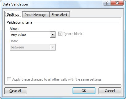
Figure 1. The Data Validation dialog box.
=INDIRECT(A3)
That's it. Now people can only select from your major list if they are using one of the cells specified in step 6, and from the appropriate dependent lists if they choose one of the cells in step 12.
There are lots of different variations of this approach (using data validation). You can find more information on some of these approaches by visiting these Web pages:
http://www.ozgrid.com/download/ (download the MatchingLists.zip file)
http://www.contextures.com/xlDataVal02.html
ExcelTips is your source for cost-effective Microsoft Excel training. This tip (10545) applies to Microsoft Excel 2007 and 2010. You can find a version of this tip for the older menu interface of Excel here: Creating Dependent Drop-Lists.

Best-Selling VBA Tutorial for Beginners Take your Excel knowledge to the next level. With a little background in VBA programming, you can go well beyond basic spreadsheets and functions. Use macros to reduce errors, save time, and integrate with other Microsoft applications. Fully updated for the latest version of Office 365. Check out Microsoft 365 Excel VBA Programming For Dummies today!
If you want to make sure that only unique values are entered in a particular column, you can use the data validation ...
Discover MoreData Validation is a great tool to make sure that data entered in a cell meets whatever criteria you decide. Its ...
Discover MoreWhen setting up Excel for data entry, you often have to be concerned with what values are acceptable. For example, if ...
Discover MoreFREE SERVICE: Get tips like this every week in ExcelTips, a free productivity newsletter. Enter your address and click "Subscribe."
2021-08-04 08:56:44
Tim Easter
Thank you, David Czuba, for taking the time to be more precise than I did with my comment. As you correctly said, data validation can only use a named range, not a table. However, you can use a structured reference to the applicable data portion of a table in your data validation so that when additional information is added to the table the named range automatically expands to include it.
In the URL given, the one-column table is named "Region", but the data portion of the table (the column of information minus the header) is named "Regionn" (note the second n), using the structured reference =Region[Region] (i.e. the column of data with the header Region in the table named Region). The data validation cells read this named range "Regionn", effectively reading whatever data is in that column of the table. If an additional column is added to this table, the named range "Regionn" will still only refer to the column with the header Region. But if more entries are added to the Region column of the table the named range "Regionn" will automatically expand to include them, thus being available in the data validation dropdown list.
To apply this to dependent dropdown lists, the named range (in the URL example, "Regionn") would have to match the entries in the initial dropdown list (e.g. "Sale", "Research", Executive" in the example given in step 4 above in the article).
2021-08-02 16:46:27
David Czuba
Thank you, Tim Easter. Just to clarify, table names cannot be used DIRECTLY as data validation lists. What is being used is a structured reference, which of course is also known as a named range. Tables 'support' structured references, which allows the INDIRECT formula to work with the table's data values. The example in the URL appears to use the column headers of the named range, however, it is the table name being used! As a test, the data validation list isn't affected if the table's column header is renamed, but it does if the table is renamed. If a second column is added to the table, the resulting data validation list includes these items in the drop-down, suggesting that the table is also stored as an array internally. I imagine the Microsoft software engineers had to compromise when supporting structured references in tables!
2021-08-02 07:50:42
Tim Easter
To make this even more useful, use tables in your data validation lists rather than named ranges. Then you can add to your lists later as needed without having to change formulas or range names (except for the primary list, which will require adding another table for the new entry).
https://sparrowsolutions.ca/datavalidationlists/
2014-03-07 04:18:59
NITIN
Thanks Bryan, I will LookUp that & Try..
2014-03-04 11:42:50
Bryan
INDEX/MATCH allows you to use tba data in one cell to look up information in a table and display it in another cell.
2014-02-28 03:06:07
Nitin
Thanks Bryan Got it & I understand your stand for not providing step-by-step instructions for free.
& Yes What you mention is exactly the same - I have only one record per name / id - not multiple order details....
You mentioned I can do it without VBA - ??? I did not understand that - do you mean there is a function to do that ?
2014-02-27 11:43:22
Bryan
As long as there is only one record per name it would be easy to use the above functions. No VBA needed. If you have multiple records attached to each name/ID in the drop down (like a customer order table -- each customer could have multiple orders) it is more complicated but the solution depend entirely on your data.
You should have to trouble finding a solution online. Off the top of my head, Chandoo.org is a good place to start. I don't want to give step by step instructions for free, especially when according to the comment policy I wouldn't what I wrote.
2014-02-27 06:41:01
Nitin
Thanks Bryan,
What I want is:
From a dropdown list in say a5, I will select a name.
Once I select the name, I would want the birthdate, spouse name, address & other data / information of THAT person to be displayed in subsequent columns designated for each piece of information.
I also intend to use the same concept for invoicing:
wherein I will select the customer id from a drop down list & on selection, automatically, the address, tax no., email id, concerned person's name etc will be filled up in the designated cells.
I would appreciate if you can give me a step by step explanation (if possible) as I am novice in macro / excel functions...
Meanwhile, I shall study the VLOOKUP & INDEX/MATCH functions.
2014-02-26 11:44:06
Bryan
Nitin, do you you want to see a whole list displayed or just one matching record? If the latter, you could simply use a VLOOKUP or an INDEX/MATCH combination.
2014-02-26 07:15:09
Nitin
Is there a way of dependant lists getting selected automatically on selection of the main list?
I mean in a drop down list (at a5), if i select a name, then a6 should display the relative details of the name - say telephone no. (from another list) & a7 should display the spouse name & a8 should display the address etc etc etc
2014-02-25 13:34:48
Bruce
Daniel. After entering the information into the cells (A2:A10 for example) highlight these cells and change the name to something relevant (like dependants) this creates the "named range" then use this name in your validation
2014-02-25 10:03:03
Daniel
I found my answer here: http://www.contextures.com/xlDataVal02.html
2014-02-25 09:56:58
Daniel
Is there some special way to create a list? When I get to step 11, I receive an error that says "A named range you specified cannot be found."
Got a version of Excel that uses the ribbon interface (Excel 2007 or later)? This site is for you! If you use an earlier version of Excel, visit our ExcelTips site focusing on the menu interface.
FREE SERVICE: Get tips like this every week in ExcelTips, a free productivity newsletter. Enter your address and click "Subscribe."
Copyright © 2026 Sharon Parq Associates, Inc.
 Please Note:
This article is written for users of the following Microsoft Excel versions: 2007 and 2010. If you are using an earlier version (Excel 2003 or earlier), this tip may not work for you. For a version of this tip written specifically for earlier versions of Excel, click here:
Please Note:
This article is written for users of the following Microsoft Excel versions: 2007 and 2010. If you are using an earlier version (Excel 2003 or earlier), this tip may not work for you. For a version of this tip written specifically for earlier versions of Excel, click here:
Comments