Extracting Numbers within a Range

Robert has a series of numbers in column A that range from 1 to 100. He would like to extract only those values between 65 and 100, inclusive, and place them in column B. He wonders if there is a way to do that easily.

The short answer is that there is a very easy way to do it, provided you don't mind sorting the list of numbers. Follow these steps:

1. Select a cell in column A. (It doesn't really matter which cell you select, as long as it is one of the cells that contains a number.)
2. Display the Data tab of the ribbon.
3. Click the Sort Smallest to Largest tool, in the Sort & Filter group. Excel sorts all the numbers in the column.
4. Select the numbers that you want to put into column B.
5. Press Ctrl+X to cut the cells to the Clipboard.
6. Select cell B1 (or the first cell in column B where you want the values to appear).
7. Press Ctrl+V to paste the cells into the column.

That's it; you've now got the desired cells into column B. If you simply wanted to copy the cells, then in step 5 you could have pressed Ctrl+C instead.

If you need to keep the values in column A in their original order (minus the values you want to move), you can do it by using column B as a "place retainer" column. To the right of the first value in column A, put the vaue 1. Then, below that in column B put a 2, then a 3, and so on, until each value in column A has a corresponding value in column B that indicates the numbers location. Then, follow these steps:

1. Select a cell in column A. (It doesn't really matter which cell you select, as long as it is one of the cells that contains a number.)
2. Display the Data tab of the ribbon.
3. Click the Sort Smallest to Largest tool, in the Sort & Filter group. Excel sorts all the numbers in the column.
4. Select the numbers in column A that you want to move, along with the numbers to the right of them in column B.
5. Press Ctrl+X to cut the cells to the Clipboard.
6. Select cell D1. (It is important to select cell D1 because you need to leave column C blank.)
7. Press Ctrl+V to paste the cells into columns D and E.
8. Select a cell in column B.
9. Display the Data tab of the ribbon.
10. Click the Sort Smallest to Largest tool, in the Sort & Filter group. Excel sorts all the numbers in the column based on the values in column B.
11. Select a cell in column E.
12. The Data tab of the ribbon should still be displayed.
13. Click the Sort Smallest to Largest tool, in the Sort & Filter group. Excel sorts all the numbers in the column based on the values in column E.
14. Delete columns B, C, and E.

At this point the values in columns A and B reflect their original order, from when they were all in column A.

Another way to move the cells is to use the filtering capabilities of Excel. Follow these steps:

1. Select a cell in column A. (It doesn't really matter which cell you select, as long as it is one of the cells that contains a number.)
2. Display the Data tab of the ribbon.
3. Click the Filter tool. Excel adds a filter drop-down arrow at the right side of the column A header.
4. Click the down-arrow and choose Number Filters | Between. Excel displays the Custom AutoFilter dialog box. (See Figure 1.)



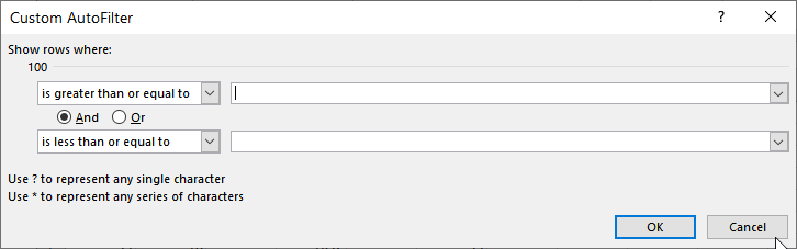
Figure 1. The Custom AutoFilter dialog box.

5. In the Greater Than or Equal To box, enter 65.
6. In the Less Than or Equal To box, enter 100.
7. Click OK. Excel limits what is shown to only those rows that meet the criteria you specified in steps 4 through 6.
8. Select the cells that are displayed.
9. Press Ctrl+C to copy the cells to the Clipboard.
10. Select cell B1 (or the first cell in column B where you want the values to appear).
11. Press Ctrl+V to paste the cells into the column.
12. Select one of the cells in column A.
13. Again click the Filter tool. (The Data tab of the ribbon should still be displayed.) Excel removes the filter you previously applied.

You could also use formulas in column B to pull out the values that are within the desired range. An easy way to do this is to place this formula in cell B1:

=IF(AND(A1>=65, A1<=100),A1,"")

Copy the formula down as far as necessary in column B and you end up with any values in the range of 65 to 100, inclusive, being "copied" into column B. If the value is outside this range, then the cell in column B is left empty.

Assuming that you don't want any empty cells in column B, then you could use an array formula to grab the values. If your values are in the range A1:A500, place the following in cell B1:

=IFERROR(INDEX(A$1:A$500,SMALL(IF(A$1:A$500>=65,ROW($1:$500)),ROW())),"")

Enter it using Ctrl+Shift+Enter, and then copy the formula down as far as you'd like.

There are, of course, macro-based solutions you can use. These are helpful if you need to perform this task quite a bit with data that you retrieve from an outside source. The following is a simple example of a macro you could use:

Sub ExtractValues1()
    Dim x As Integer

    x = 1
    For Each cell In Selection
        If cell.Value >= 65 And cell.Value <= 100 Then
            Cells(x, 2) = cell.Value
            x = x + 1
        End If
    Next cell
End Sub

You use the macro by selecting the cells you want evaluated in column A and then running it. It looks at each cell and copies the value to column B. The original value in column A is left unchanged.

For more flexibility you could rely on asking the user for the lower and upper values, as shown in this macro:

Sub ExtractValues2()
    Dim iLowVal As Integer
    Dim iHighVal As Integer

    iLowVal = InputBox("Lowest value wanted?")
    iHighVal = InputBox("Highest value wanted?")

    For Each cell In Range("A:A")
        If cell.Value <= iHighVal And cell.Value >= iLowVal Then
            ActiveCell.Value = cell.Value
            ActiveCell.Offset(1, 0).Activate
        End If
    Next
End Sub

Before you run the macro, select the cell at the top of the range where you want the extracted values placed. Nothing in column A is affected; only the values between the lower and upper range are copied to the new location.

ExcelTips is your source for cost-effective Microsoft Excel training. This tip (13397) applies to Microsoft Excel 2007, 2010, 2013, 2016, 2019, and Excel in Microsoft 365.